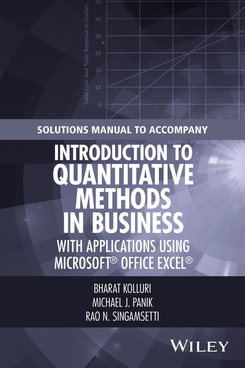
Solutions Manual to Accompany Introduction to Quantitative Methods in Business: with Applications Using Microsoft Office Excel (eBook)
John Wiley & Sons (Verlag)
978-1-119-22104-3 (ISBN)
Bharat Kolluri, PhD, is Professor of Economics in the Department of Economics, Finance, and Insurance at the University of Hartford. A member of the American Economics Association, his research interests include econometrics, business statistics, quantitative decision making, applied macroeconomics, applied microeconomics, and corporate finance. Michael J. Panik, PhD, is Professor Emeritus in the Department of Economics, Finance, and Insurance at the University of Hartford. He has served as a consultant to the Connecticut Department of Motor Vehicles as well as to a variety of healthcare organizations. In addition, Dr. Panik is the author of numerous books including Growth Curve Modeling: Theory and Applicationsand Statistical Inference: A Short Course, both published by Wiley. Rao N. Singamsetti, PhD, is Associate Professor in the Department of Economics, Finance, and Insurance at the University of Hartford. A member of the American Economics Association, his research interests include the status of war on poverty in the United States since the 1960's and forecasting foreign exchange rates using econometric methods.
1. The Mathematical Toolbox: A Summary 1
1.2 Linear Functions 1
1.3.1 Solving Two Simultaneous Linear Equations 1
1.4 Summation Notation 2
1.5 Sets 3
1.6 Functions and Graphs 3
1.7 Working with Functions 4
1.8 Differentiation and Integration 5
Solutions to Odd-Numbered Exercises 8
2. Applications of Linear and Nonlinear Functions: A Summary 32
2.2 Linear Demand and Supply Functions 32
2.3 Linear Total Cost and Total Revenue Functions 33
2.4 Market Equilibrium 33
2.6 Applications of Nonlinear Functions 34
2.7 Present Value of an Income Stream 35
2.8 Average Values 35
2.9 Marginal Values 36
2.10 Elasticity 36
Solutions to Odd-Numbered Exercises 37
3. Optimization: A Summary 47
3.2 Unconstrained Optimization 47
3.2.1 Models of Profit and Revenue Maximization 47
3.2.3 Solution Using the Calculus Approach 47
3.2.5 Solution Using the Calculus Approach 47
3.3 Models of Cost Minimization: Inventory Cost Functions and Economic Order Quantity (EOQ) 48
3.3.2 Solution Using the Calculus Approach 49
3.4 Constrained Optimization: Linear Programming 50
3.4.1 Linear Programming: Maximization 50
3.4.2 Linear Programming: Minimization 51
Solutions to Odd-Numbered Exercises 52
4. What Is Business Statistics? 68
4.3 Descriptive Statistics: Tabular and Graphical Techniques 68
4.4 Descriptive Statistics: Numerical Measures of Central Tendency or Location of Data 70
4.4.1 Population Mean 70
4.4.2 Sample Mean 70
4.4.3 Weighted Mean 70
4.4.4 Mean of a Frequency Distribution: Grouped Data 71
4.4.5 Geometric Mean 71
4.4.6 Median 71
4.4.7 Quantiles, Quartiles, Deciles, and Percentiles 71
4.4.8 Mode 72
4.5 Descriptive Statistics: Measures of Dispersion (Variability or Spread) 73
4.5.2 Variance 73
4.5.3 Standard Deviation 74
4.5.4 Coefficient of Variation 74
4.5.5 Some Important Uses of the Standard Deviation 75
1. Standardization of Values 75
2. Chebysheff's Theorem 75
4.5.6 Empirical Rule 75
4.6 Measuring Skewness 76
Solutions to Odd-Numbered Exercises 76
5. Probability and Applications 96
5.2 Some Useful Definitions 96
5.3 Probability Sources 96
5.3.1 Objective Probability 96
5.4 Some Useful Definitions Involving Sets of Events in the Sample Space 96
5.5 Probability Laws 97
5.5.2 Rule of Complements 97
5.5.3 Conditional Probability 97
5.5.4 General Multiplication Rule (Product Rule) 97
5.5.5 Independent Events 98
5.5.6 Probability Tree Approach 98
5.6 Contingency Table 98
Solutions to Odd-Numbered Exercises 100
6. Random Variables and Probability Distributions 105
6.2 Probability Distribution of a Discrete Random Variable X 105
6.3 Expected Value, Variance, and Standard Deviation of a Discrete Random Variable 106
6.3.1 Some Basic Rules of Expectation 106
6.3.2 Some Useful Properties of the Variance of X 107
6.4 Continuous Random Variables and Their Probability Distributions 107
6.5 A Specific Discrete Probability Distribution: The Binomial Case 108
6.5.1 Binomial Probability Distribution 108
6.5.2 Mean and Standard Deviation of the Binomial Random Variable 109
6.5.3 Cumulative Binomial Probability Distribution 110
Solutions to Odd-Numbered Exercises 110
Index 119
Chapter 1
The Mathematical Toolbox: A Summary
1.2 Linear Functions
An expression such as represents a linear equation (function), where is the Y-intercept (it gives the value of Y when X = 0) and is the slope (often referred to as rise/run). Here Y is the dependent variable and X is the independent variable. Note that both and are constants.
1.3.1 Solving Two Simultaneous Linear Equations
At times you will need to obtain a solution to a set of simultaneous linear equations, that is, to a set of equations of the general form:
A system such as this is said to be consistent if it has at least one solution. Moreover, if , then this equation system is consistent. For instance, the equation system
is consistent since (1) (−2) − (3) (−1) = 1 ≠ 0. In fact, to obtain the (unique) solution, we can multiply (Equation 1.3) by −3 so as to obtain −3X + 3Y = −18, and then add this multiple to (Equation 1.4) to get Y = −14. If we then substitute Y = −14 into (Equation 1.3), we obtain X = −8. How do we know that we have generated the correct solution to this equation system?
Answer: Substitute X = −8 and Y = −14 back into, say, (Equation 1.4) and show that equality holds.
It is easily demonstrated that the equation system
is inconsistent or dependent in that it has no solution. Here (4) (8) − (16) (2) = 0. Clearly, these two equations represent parallel lines—they do not intersect.
1.4 Summation Notation
The operation of addition of a set of n values is readily carried out by using the “sigma” notation. In this regard, the left-hand side of the expression
reads: “the sum of all values as i goes from 1 to n.” The right-hand side shows that the operation of addition has been executed. Some useful summation rules are as follows:
- Rule 1:
- Rule 2: , where c is a constant.
- Rule 3: where c is a constant.
Note also that
if is the sample mean, then
The Pearson sample correlation coefficient can be written as either
where and are the sample means of X and Y, respectively; or as
Given a collection of data points we can fit a linear equation of the form Y = a + bX through them, where a is the Y-intercept and b is the slope. Here,
or
and .
1.5 Sets
We know that a set is a collection or grouping of items (called elements) without regard to structure or order and that a set is usually defined by listing its elements. A set containing no elements is called the null set or the empty set and is denoted as ϕ. A set containing all elements under a particular discussion or in a given context is termed the universal set and is denoted as U. Given a set A, its complement, denoted , is the set containing all the elements within U that lie outside of A.
The intersection of two sets A and B is the set of elements common to both A and B. It is denoted as . The union of two sets A and B contains the elements in A, or in B, or in both A and B. It is denoted as . A moments reflection reveals the following:
1.6 Functions and Graphs
A function f is a rule or law of correspondence that associates with each value of a variable x a unique value of a variable y. Here y is termed the image of x under rule f. This “rule” is written as y = f (x) and is read: “y is a function of x.” Think of a function as a recipe for getting unique y values from x values. Here x is termed the independent variable and y is called the dependent variable. The set of all admissible x values is called the domain of the function; the collection of y values, which are the image of at least one x, is termed the range of the function. For instance, a function may appear as . What is the rule that is operative here? The rule is: Select a value of x, multiply it by itself, and then add 2 to the result to get y. So, if x = 2, the image of x = 2 via rule f is
It is important to note that for each x value there is one and only one resulting value of y. However, a y value may be the image of more than one x value. However, if implies , then f is said to be a one-to-one function.
A useful device for illustrating a function is its graph. Here y is plotted on the vertical axis and x is plotted on the horizontal axis. Then, via the rule f, a set of x values are chosen and their corresponding y values are determined. These ordered (x, y) combinations are then connected to form the graph of the function in the x–y-plane (see Figure 1.1).
Figure 1.1 The graph of the function y = f(x) = x2.
Given a particular graph, how can we determine whether or not it represents a function?
Answer: We can employ the vertical line test: For a given value of x, find y by drawing a vertical line at x. If the line cuts the graph at only a single value of y, then the graph indeed represents a function.
1.7 Working with Functions
At times it is important to be able to graph a linear function in a quick and efficient fashion. To this end, let us consider the following approach:
- Intercept method: Since two points are enough to draw a unique straight line, find both the horizontal intercept (set y = 0 and solve for the x-intercept) and the vertical intercept (set x = 0 and solve for the y-intercept) and connect the resulting two points, which are called basic points. For instance, suppose y = 2x − 6. Then,
- if y = 0, then 2x − 6 = 0 or x = 3; and
- if x = 0, then y = −6.
Hence, the two basic points are (3, 0) and (0, −6). These points are then connected to obtain the desired graph.
An alternative method for graphing a function (which is useful for both linear and nonlinear equations) is the point method:
- Point method: Given an admissible set of x values, we use the rule f to get the corresponding y values and then we connect each of the resulting ordered pairs (x, y) (see Figure 1.1).
1.8 Differentiation and Integration
We may think of a function as being continuous if its graph is without breaks. Additionally, the derivative of a function y = f(x) with respect to x is defined as
Here dy/dx is the instantaneous rate of change in y per unit change in x as Δx gets smaller and smaller. Note that if f has a derivative at a point x = a, then it is also continuous at x = a. However, if f is continuous at a point x = a, it does not follow that f has a derivative there.
The derivative is also interpreted as the slope of the function y = f(x) at a given point, that is, for x = a, is the slope of f at this x value. Additionally, depicts the marginal change in y with respect to x.
Rules of Differentiation:
- Power rule: If , then . (If .)
- The derivative of a constant is zero.
- Coefficient rule: If , then . (If , then . Here, k = 6 and .)
- Sum (difference) rule: If , then . (If , then .)
- Product rule: If , then . (If , then .)
- Quotient rule: If , then
(If , then )
- Derivatives of exponential and logarithmic functions:
- If .
- If , where k is a constant.
- If .
Higher Order Derivatives:
- Given that the first derivative of f with respect to x appears as , the second derivative of f with respect to x is written as and is calculated as the derivative of the first derivative.
(If .)
Geometrically, the second derivative of f is the rate of change of the slope of f at a specific point on the graph of f. For instance, at a point x = a, if , then f is said to be concave downward at x = a; and if , then f is termed concave upward of x = a.
- The third derivative of f with respect to x is the derivative of the second derivative. (Given above, .)
- In general, the nth order derivative of f with respect to x is the derivative of the (n − 1)th order derivative, for example, the sixth derivative of f is the derivative of the fifth derivative of f.
There are two distinct ways to view the concept of an integral. On the one hand, we have the definite integral—an integral that is the limit of an...
| Erscheint lt. Verlag | 7.7.2016 |
|---|---|
| Sprache | englisch |
| Themenwelt | Informatik ► Office Programme ► Excel |
| Mathematik / Informatik ► Mathematik ► Angewandte Mathematik | |
| Mathematik / Informatik ► Mathematik ► Finanz- / Wirtschaftsmathematik | |
| Mathematik / Informatik ► Mathematik ► Statistik | |
| Mathematik / Informatik ► Mathematik ► Wahrscheinlichkeit / Kombinatorik | |
| Technik | |
| Wirtschaft | |
| Schlagworte | Arithmetic Operations • business • Business & Corporate Economics • Business & Management • business applications • Business Statistics • Business Statistics & Math • corporate economics • Data Analysis • descriptive statistics • discrete and continuous random variables • Economics • elementary differentiations • Finance • Finanz- u. Wirtschaftsstatistik • formulae usage • Functions and Graphs • Graphing • Integration • linear and nonlinear models • Marketing • Mathematics • operations • Optimization • Quantitative Methoden • Quantitative Methods • quantitative techniques • rates of change • solving equations • Statistics • Statistics for Finance, Business & Economics • Statistik • Volks- u. Betriebswirtschaftslehre • Volkswirtschaftslehre • Wirtschaftsmathematik • Wirtschaftsmathematik u. -statistik • Wirtschaftsstatistik • Wirtschaft u. Management |
| ISBN-10 | 1-119-22104-8 / 1119221048 |
| ISBN-13 | 978-1-119-22104-3 / 9781119221043 |
| Informationen gemäß Produktsicherheitsverordnung (GPSR) | |
| Haben Sie eine Frage zum Produkt? |
Größe: 16,0 MB
Kopierschutz: Adobe-DRM
Adobe-DRM ist ein Kopierschutz, der das eBook vor Mißbrauch schützen soll. Dabei wird das eBook bereits beim Download auf Ihre persönliche Adobe-ID autorisiert. Lesen können Sie das eBook dann nur auf den Geräten, welche ebenfalls auf Ihre Adobe-ID registriert sind.
Details zum Adobe-DRM
Dateiformat: PDF (Portable Document Format)
Mit einem festen Seitenlayout eignet sich die PDF besonders für Fachbücher mit Spalten, Tabellen und Abbildungen. Eine PDF kann auf fast allen Geräten angezeigt werden, ist aber für kleine Displays (Smartphone, eReader) nur eingeschränkt geeignet.
Systemvoraussetzungen:
PC/Mac: Mit einem PC oder Mac können Sie dieses eBook lesen. Sie benötigen eine
eReader: Dieses eBook kann mit (fast) allen eBook-Readern gelesen werden. Mit dem amazon-Kindle ist es aber nicht kompatibel.
Smartphone/Tablet: Egal ob Apple oder Android, dieses eBook können Sie lesen. Sie benötigen eine
Geräteliste und zusätzliche Hinweise
Buying eBooks from abroad
For tax law reasons we can sell eBooks just within Germany and Switzerland. Regrettably we cannot fulfill eBook-orders from other countries.
Kopierschutz: Adobe-DRM
Adobe-DRM ist ein Kopierschutz, der das eBook vor Mißbrauch schützen soll. Dabei wird das eBook bereits beim Download auf Ihre persönliche Adobe-ID autorisiert. Lesen können Sie das eBook dann nur auf den Geräten, welche ebenfalls auf Ihre Adobe-ID registriert sind.
Details zum Adobe-DRM
Dateiformat: EPUB (Electronic Publication)
EPUB ist ein offener Standard für eBooks und eignet sich besonders zur Darstellung von Belletristik und Sachbüchern. Der Fließtext wird dynamisch an die Display- und Schriftgröße angepasst. Auch für mobile Lesegeräte ist EPUB daher gut geeignet.
Systemvoraussetzungen:
PC/Mac: Mit einem PC oder Mac können Sie dieses eBook lesen. Sie benötigen eine
eReader: Dieses eBook kann mit (fast) allen eBook-Readern gelesen werden. Mit dem amazon-Kindle ist es aber nicht kompatibel.
Smartphone/Tablet: Egal ob Apple oder Android, dieses eBook können Sie lesen. Sie benötigen eine
Geräteliste und zusätzliche Hinweise
Buying eBooks from abroad
For tax law reasons we can sell eBooks just within Germany and Switzerland. Regrettably we cannot fulfill eBook-orders from other countries.
aus dem Bereich
