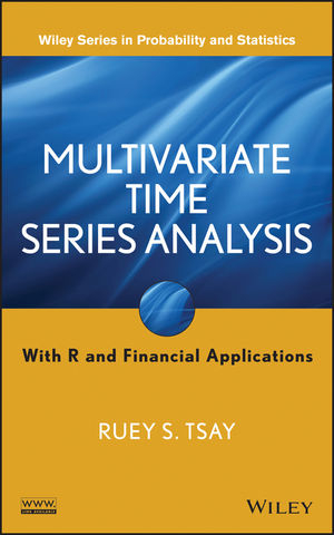
Multivariate Time Series Analysis (eBook)

With R and Financial Applications

Ruey S. Tsay (Autor)

eBook Download: EPUB

2013 | 1. Auflage
520 Seiten
John Wiley & Sons (Verlag)
978-1-118-61775-5 (ISBN)

Infos

An accessible guide to the multivariate time series tools
used in numerous real-world applications

Multivariate Time Series Analysis: With R and Financial
Applications is the much anticipated sequel coming from one of
the most influential and prominent experts on the topic of time
series. Through a fundamental balance of theory and methodology,
the book supplies readers with a comprehensible approach to
financial econometric models and their applications to real-world
empirical research.

Differing from the traditional approach to multivariate time
series, the book focuses on reader comprehension by emphasizing
structural specification, which results in simplified parsimonious
VAR MA modeling. Multivariate Time Series Analysis: With R and
Financial Applications utilizes the freely available R
software package to explore complex data and illustrate related
computation and analyses. Featuring the techniques and methodology
of multivariate linear time series, stationary VAR models, VAR MA
time series and models, unitroot process, factor models, and
factor-augmented VAR models, the book includes:

* Over 300 examples and exercises to reinforce the
presented content

* User-friendly R subroutines and research presented
throughout to demonstrate modern applications

* Numerous datasets and subroutines to provide readers
with a deeper understanding of the material

Multivariate Time Series Analysis is an ideal textbook
for graduate-level courses on time series and quantitative finance
and upper-undergraduate level statistics courses in time series.
The book is also an indispensable reference for researchers and
practitioners in business, finance, and econometrics.

Autor

RUEY S. TSAY, PhD, is H.G.B. Alexander Professor of Econometrics and Statistics at The University of Chicago Booth School of Business. He has written over 125 published articles in the areas of business and economic forecasting, data analysis, risk management, and process control. A Fellow of the American Statistical Association, the Institute of Mathematical Statistics, and Academia Sinica, Dr. Tsay is author of Analysis of Financial Time Series, Third Edition and An Introduction to Analysis of Financial Data with R, and coauthor of A Course in Time Series Analysis, all published by Wiley.

Inhalt

Preface xv

Acknowledgements xvii

1 Multivariate Linear Time Series 1

1.1 Introduction, 1

1.2 Some Basic Concepts, 5

1.3 Cross-Covariance and Correlation Matrices, 8

1.4 Sample CCM, 9

1.5 Testing Zero Cross-Correlations, 12

1.6 Forecasting, 16

1.7 Model Representations, 18

1.8 Outline of the Book, 22

1.9 Software, 23

Exercises, 23

2 Stationary Vector Autoregressive Time Series 27

2.1 Introduction, 27

2.2 VAR(1) Models, 28

2.3 VAR(2) Models, 37

2.4 VAR(p) Models, 41

2.5 Estimation, 44

2.6 Order Selection, 61

2.7 Model Checking, 66

2.8 Linear Constraints, 80

2.9 Forecasting, 82

2.10 Impulse Response Functions, 89

2.11 Forecast Error Variance Decomposition, 96

2.12 Proofs, 98

Exercises, 100

3 Vector Autoregressive Moving-Average Time Series 105

3.1 Vector MA Models, 106

3.2 Specifying VMA Order, 112

3.3 Estimation of VMA Models, 113

3.4 Forecasting of VMA Models, 126

3.5 VARMA Models, 127

3.6 Implications of VARMA Models, 139

3.7 Linear Transforms of VARMA Processes, 141

3.8 Temporal Aggregation of VARMA Processes, 144

3.9 Likelihood Function of a VARMA Model, 146

3.10 Innovations Approach to Exact Likelihood Function, 155

3.11 Asymptotic Distribution of Maximum Likelihood Estimates, 160

3.12 Model Checking of Fitted VARMA Models, 163

3.13 Forecasting of VARMA Models, 164

3.14 Tentative Order Identification, 166

3.15 Empirical Analysis of VARMA Models, 176

3.16 Appendix, 192

Exercises, 194

4 Structural Specification of VARMA Models 199

4.1 The Kronecker Index Approach, 200

4.2 The Scalar Component Approach, 212

4.3 Statistics for Order Specification, 220

4.4 Finding Kronecker Indices, 222

4.5 Finding Scalar Component Models, 226

4.6 Estimation, 237

4.7 An Example, 245

4.8 Appendix: Canonical Correlation Analysis, 259

Exercises, 262

5 Unit-Root Nonstationary Processes 265

5.1 Univariate Unit-Root Processes, 266

5.2 Multivariate Unit-Root Processes, 279

5.3 Spurious Regressions, 290

5.4 Multivariate Exponential Smoothing, 291

5.5 Cointegration, 294

5.6 An Error-Correction Form, 297

5.7 Implications of Cointegrating Vectors, 300

5.8 Parameterization of Cointegrating Vectors, 302

5.9 Cointegration Tests, 303

5.10 Estimation of Error-Correction Models, 313

5.11 Applications, 319

5.12 Discussion, 326

5.13 Appendix, 327

Exercises, 328

6 Factor Models and Selected Topics 333

6.1 Seasonal Models, 333

6.2 Principal Component Analysis, 341

6.3 Use of Exogenous Variables, 345

6.4 Missing Values, 357

6.5 Factor Models, 364

6.6 Classification and Clustering Analysis, 386

Exercises, 394

7 Multivariate Volatility Models 399

7.1 Testing Conditional Heteroscedasticity, 401

7.2 Estimation of Multivariate Volatility Models, 407

7.3 Diagnostic Checks of Volatility Models, 409

7.4 Exponentially Weighted Moving Average, 414

7.5 BEKK Models, 417

7.6 Cholesky Decomposition and Volatility Modeling, 420

7.7 Dynamic Conditional Correlation Models, 428

7.8 Orthogonal Transformation, 434

7.9 Copula-Based Models, 443

7.10 Principal Volatility Components, 454

Exercises, 461

Appendix A Review of Mathematics and Statistics 465

A.1 Review of Vectors and Matrices, 465

A.2 Least-Squares Estimation, 477

A.3 Multivariate Normal Distributions, 478

A.4 Multivariate Student-t Distribution, 479

A.5 Wishart and Inverted Wishart Distributions, 480

A.6 Vector and Matrix Differentials, 481

Index 489

Produkt-Details

• Erscheint lt. Verlag: 11.11.2013
• Reihe/Serie: Wiley Series in Probability and Statistics
• Reihe/Serie: Wiley Series in Probability and Statistics
• Sprache: englisch
• Themenwelt: Mathematik / Informatik ► Mathematik ► Analysis
• Themenwelt: Mathematik / Informatik ► Mathematik ► Statistik
• Themenwelt: Mathematik / Informatik ► Mathematik ► Wahrscheinlichkeit / Kombinatorik
• Themenwelt: Technik
• Themenwelt: Wirtschaft ► Volkswirtschaftslehre
• Schlagworte: Ökonometrie • Econometrics • Economics • Multivariate Analyse • multivariate analysis • Ökonometrie • Statistics • Statistik • Time Series • Volkswirtschaftslehre • Zeitreihen • Zeitreihenanalyse
• ISBN-10: 1-118-61775-4 / 1118617754
• ISBN-13: 978-1-118-61775-5 / 9781118617755