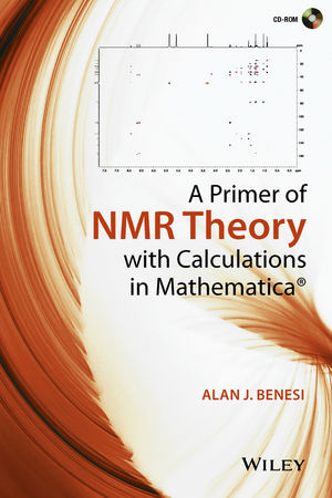
A Primer of NMR Theory with Calculations in Mathematica (eBook)
John Wiley & Sons (Verlag)
978-1-119-05199-2 (ISBN)
- Provides short, focused chapters with brief explanations of well-defined topics with an emphasis on a mathematical description
- Presents essential results from quantum mechanics concisely and for easy use in predicting and simulating the results of NMR experiments
- Includes Mathematica notebooks that implement the theory in the form of text, graphics, sound, and calculations
- Based on class tested methods developed by the author over his 25 year teaching career. These notebooks show exactly how the theory works and provide useful calculation templates for NMR researchers
Alan J. Benesi was Director of the Pennsylvania State University NMR Facility from 1987-2012. He earned his Ph.D. in Biophysics at the University of California, Berkeley, in 1975. He has published many papers related to solid state and liquid state NMR, solid state and liquid state NMR relaxation, and rotational and translational diffusion.
Presents the theory of NMR enhanced with Mathematica notebooks Provides short, focused chapters with brief explanations of well-defined topics with an emphasis on a mathematical description Presents essential results from quantum mechanics concisely and for easy use in predicting and simulating the results of NMR experiments Includes Mathematica notebooks that implement the theory in the form of text, graphics, sound, and calculations Based on class tested methods developed by the author over his 25 year teaching career. These notebooks show exactly how the theory works and provide useful calculation templates for NMR researchers
Alan J. Benesi was Director of the Pennsylvania State University NMR Facility from 1987-2012. He earned his Ph.D. in Biophysics at the University of California, Berkeley, in 1975. He has published many papers related to solid state and liquid state NMR, solid state and liquid state NMR relaxation, and rotational and translational diffusion.
Preface viii
Chapter 1 Introduction 1
Chapter 2 Using Mathematicac; Homework Philosophy 3
Chapter 3 The NMR Spectrometer 4
Chapter 4 The NMR Experiment 7
Chapter 5 Classical Magnets and Precession 11
Chapter 6 The Bloch Equation in the Laboratory Reference Frame 16
Chapter 7 The Bloch Equation in the Rotating Frame 19
Chapter 8 The Vector Model 23
Chapter 9 Fourier Transform of the NMR Signal 29
Chapter 10 Essentials of Quantum Mechanics 31
Chapter 11 The Time?]Dependent Schrodinger Equation, Matrix Representation of Nuclear Spin Angular Momentum Operators 35
Chapter 12 The Density Operator 39
Chapter 13 The Liouville-von Neumann Equation 41
Chapter 14 The Density Operator at Thermal Equilibrium 42
Chapter 15 Hamiltonians of NMR: Isotropic Liquid?]State Hamiltonians 45
Chapter 16 The Direct Product Matrix Representation of Coupling Hamiltonians HJ and HD 50
Chapter 17 Solving the Liouville-Von Neumann Equation for the Time Dependence of the Density Matrix 54
Chapter 18 The Observable NMR Signal 59
Chapter 19 Commutation Relations of Spin Angular Momentum Operators 61
Chapter 20 The Product Operator Formalism 65
Chapter 21 NMR Pulse Sequences and Phase Cycling 68
Chapter 22 Analysis of Liquid?]State NMR Pulse Sequences with the Product Operator Formalism 72
Chapter 23 Analysis of the Inept Pulse Sequence with Program Shortspin and Program Poma 78
Chapter 24 The Radio Frequency Hamiltonian 82
Chapter 25 Comparison of 1D and 2D NMR 86
Chapter 26 Analysis of the HSQC, HMQC, and DQF?]COSY 2D NMR Experiments 89
Chapter 27 Selection of Coherence Order Pathways with Phase Cycling 96
Chapter 28 Selection of Coherence Order Pathways with Pulsed Magnetic Field Gradients 104
Chapter 29 Hamiltonians of NMR: Anisotropic Solid?]State Internal Hamiltonians in Rigid Solids 111
Chapter 30 Rotations of Real Space Axis Systems--Cartesian Method 120
Chapter 31 Wigner Rotations of Irreducible Spherical Tensors 123
Chapter 32 Solid?]State NMR Real Space Spherical Tensors 129
Chapter 33 Time?]Independent Perturbation Theory 134
Chapter 34 Average Hamiltonian Theory 141
Chapter 35 The Powder Average 144
Chapter 36 Overview of Molecular Motion and NMR 147
Chapter 37 Slow, Intermediate, And Fast Exchange In Liquid?]State Nmr Spectra 150
Chapter 38 Exchange in Solid?]State NMR Spectra 154
Chapter 39 N MR Relaxation: What is NMR Relaxation and what Causes it? 163
Chapter 40 Practical Considerations for the Calculation of NMR Relaxation Rates 168
Chapter 41 The Master Equation for NMR Relaxation--Single Spin Species I 170
Chapter 42 Heteronuclear Dipolar and J Relaxation 183
Chapter 43 Calculation of Autocorrelation Functions, Spectral Densities, and NMR Relaxation Times for Jump Motions in Solids 189
Chapter 44 Calculation of Autocorrelation Functions and Spectral Densities for Isotropic Rotational Diffusion 198
Chapter 45 Conclusion 202
Bibliography 203
INDEX 000
CHAPTER 5
CLASSICAL MAGNETS AND PRECESSION
In some ways, NMR active nuclei behave like classical magnetic dipoles. The classical description of magnetic dipoles in an externally applied magnetic field is therefore presented in this chapter.
In the classical view of NMR, the nucleus is likened to a sphere of charge +z (the atomic number, i.e., the number of protons in the nucleus) and mass m spinning about its z axis. The spinning mass has spin angular momentum, and the spinning charge generates a magnetic dipole moment proportional to and parallel to the spin angular momentum vector as illustrated in Figure 5.1.
Figure 5.1 Classical magnetic dipole moment μ of a spinning charged particle.
Let Ze be the charge of the nucleus, where Z is the atomic number (number of protons) and e is the proton charge. Let m be the mass of the nucleus, c be the speed of light, L be the angular momentum vector, and μ be the resulting magnetic dipole moment vector chosen arbitrarily to define the z axis. L and μ are vectors, denoted in boldface. The derivation yields the following (Gerstein, 2002):
This equation predicts that the magnetic moment is proportional to the nuclear spin angular momentum (true) but also predicts that the gyromagnetic ratio γ increases with the spin angular momentum and charge of the nucleus (false).
Some other experimental observations are incompatible with the predictions of the classical model. If a classical model held, one would not expect the angular momentum to be quantized. Moreover, the classical result predicts a single energy “level” proportional to the dot product of the magnetic moment and the applied magnetic field, disallowing transitions (see Eq. 5.2). Therefore, one would not expect to observe interactions at a single Larmor frequency for a given NMR-observable isotope. Despite these shortcomings, the classical model describes some aspects of NMR very accurately, for example, the effect of applied magnetic fields and radio frequency irradiation on nuclei in the liquid state.
In the presence of the external NMR magnetic field B = {0,0,B0}, the classical behavior of the nuclear spin magnetic dipoles μ is described by the following equation:
where × represents the vector cross product. The resulting motion is precession of the nuclear magnetic dipole moment μ around the magnetic field B (see Fig. 5.2), with a positive rotation around the field defined by the right-hand rule. The right-hand rule works as follows: Take your right hand. Align your thumb with B pointing toward the north pole of the magnet. The direction of motion of μ around your thumb is indicated by your remaining fingers, illustrated in Figure 5.2.
Figure 5.2 Precession of a magnetic dipole moment μ around a magnetic field B.
The energy of μ in radians s−1 (i.e., units of h/2π) in the magnetic field B relative to no magnetic field is as follows:
The problem with this result is that there is only one energy “level,” so no transitions can occur.
Equation 5.2 is the basis of the Bloch equation(s), which are widely used in NMR calculations for I = 1/2 nuclei and for quadrupolar nuclei in liquids (that behave like I = 1/2 nuclei). The Mathematica notebook magdipoleanimation.nb goes through the mathematics and provides animation of a classical magnetic dipole precessing in a permanent magnetic field B.
EXPLANATION OF MATHEMATICA PROGRAMMING IN magdipoleanimation.nb
The first input line of magdipoleanimation.nb is a comment of the form (* comment *). On the right-hand side of the Mathematica notebook, the input of the comment is denoted by a closing square bracket with a small diagonal from the upper left-hand side of the bracket to the right-hand vertical part of the bracket. All Mathematica input lines are indicated in this way. Comments are input by typing a left parenthesis and *, typing the comment, then finishing with a * and right parenthesis. All input lines in Mathematica are evaluated by typing shift Enter on the qwertyuiop keypad or typing enter on the numeric keypad (far right-hand-side bottom key).
The next input line demonstrates how a symbol, in this case a vector μ representing the magnetic dipole moment vector, is defined. In Mathematica, symbols such as μ are most easily chosen using the Basic Math Input palette. This palette is activated by clicking on Palettes → Other → Basic Math Input. By using the equal sign, μ is defined as a vector with time-dependent Cartesian coordinates µx[t], µy[t], and µz[t]. The vector is indicated by the left- and right-hand squiggly brackets, { and }. In this case, the input line generates an output line, denoted on the right-hand side of the notebook by a closing square bracket, small diagonal from upper left- to the right-hand vertical part, and a small mark projecting left at right angles to the vertical part. All Mathematica output lines are indicated in this way. The output line gives the evaluation result of the input line, in this case a restatement of the input definition. The combination of the input and output lines is called a “cell” and is indicated on the right-hand side of the notebook by the large closing square bracket enclosing the smaller input and output square brackets. Input lines, output lines, and entire cells can be copied by highlighting the respective brackets, then typing ctrl/c. They can be inserted after copying by putting the mouse cursor below another cell, then typing ctrl/v.
The next input line is a comment and generates no output.
The next input line defines the permanent magnetic field vector B. It generates an output line that restates the input definition.
Mathematica has a huge number of built-in functions. The next cell demonstrates the function MatrixForm. The input line requests the matrix form of the magnetic dipole vector μ. The built-in function MatrixForm yields the output line showing the three time-dependent elements of the μ vector as a column vector. This form is more consistent with mathematical convention than the squiggly bracket form.
The next cell generates the matrix form of the permanent magnetic field vector.
The next input line is a comment.
The next cell defines a variable dμdt that expresses the rate of change of the magnetic dipole moment. Here, γ is the gyromagnetic ratio of the nucleus, μ is the magnetic dipole moment vector, × is the cross product operation, and B is the permanent magnetic field vector. The output line shows that dμdt is a vector with x, y, and z components B0 γ µy[t], −B0 γ µx[t], and 0 respectively.
The next input line is a comment.
One of the very useful aspects of Mathematica is that the different parts of an expression can be “extracted” by specifying the part number. The next cell extracts the first part (the x component) of the vector dμdt, yielding B0 γ µy[t]. Extraction of the parts of an expression is achieved by enclosing the desired part between double square brackets.
The next cell extracts the second part (the y component) of the vector dμdt, yielding −B0 γ µx[t].
The next cell extracts the third part (the z component) of the vector dμdt, yielding 0.
The next input line is a comment.
The next cell shows how for all built-in Mathematica functions, information about the function can be obtained by typing? function, in this case ?/. . More detailed information can be obtained by clicking on the >> in the output line of the cell. In this book, /. is called the substitution function.
The next cell demonstrates how the substitution function is used in Mathematica. It defines a new symbol, dμdtω0, that is obtained from dμdt by substituting the negative Larmor frequency −ω0 for the product B0 γ. The substitution is carried out with the built-in /. command. The input line for this cell can be interpreted as “define a new symbol dμdtω0 that is equal to the symbol dμdt such that all occurrences of the product B0 γ (or γ B0) are replaced with −ω0.” The resulting output line shows the successful result.
The next input line is a comment.
The next cell introduces the built-in Mathematica function DSolve, which is used to solve differential equations.
The next input line can be read as solve the set of differential...
| Erscheint lt. Verlag | 19.5.2015 |
|---|---|
| Sprache | englisch |
| Themenwelt | Naturwissenschaften ► Chemie ► Analytische Chemie |
| Naturwissenschaften ► Physik / Astronomie ► Elektrodynamik | |
| Technik | |
| Schlagworte | Chemie • Chemistry • NMR, NMR theory, solid state NMR, NMR relaxation, NMR pulse sequences, NMR simulations, Molecular Motion and NMR, Density Operator, Density Matrix, Wigner rotations, spherical tensors, product operator theory, jump motions in solids, rotational diffusion in liquids • NMR Spectroscopy / MRI / Imaging • NMR-Spektroskopie • NMR-Spektroskopie / MRT / Bildgebende Verfahren • Organic Chemistry • Organische Chemie • Physics • Physik |
| ISBN-10 | 1-119-05199-1 / 1119051991 |
| ISBN-13 | 978-1-119-05199-2 / 9781119051992 |
| Informationen gemäß Produktsicherheitsverordnung (GPSR) | |
| Haben Sie eine Frage zum Produkt? |
Kopierschutz: Adobe-DRM
Adobe-DRM ist ein Kopierschutz, der das eBook vor Mißbrauch schützen soll. Dabei wird das eBook bereits beim Download auf Ihre persönliche Adobe-ID autorisiert. Lesen können Sie das eBook dann nur auf den Geräten, welche ebenfalls auf Ihre Adobe-ID registriert sind.
Details zum Adobe-DRM
Dateiformat: EPUB (Electronic Publication)
EPUB ist ein offener Standard für eBooks und eignet sich besonders zur Darstellung von Belletristik und Sachbüchern. Der Fließtext wird dynamisch an die Display- und Schriftgröße angepasst. Auch für mobile Lesegeräte ist EPUB daher gut geeignet.
Systemvoraussetzungen:
PC/Mac: Mit einem PC oder Mac können Sie dieses eBook lesen. Sie benötigen eine
eReader: Dieses eBook kann mit (fast) allen eBook-Readern gelesen werden. Mit dem amazon-Kindle ist es aber nicht kompatibel.
Smartphone/Tablet: Egal ob Apple oder Android, dieses eBook können Sie lesen. Sie benötigen eine
Geräteliste und zusätzliche Hinweise
Buying eBooks from abroad
For tax law reasons we can sell eBooks just within Germany and Switzerland. Regrettably we cannot fulfill eBook-orders from other countries.
aus dem Bereich


