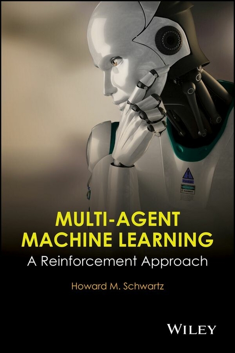
Multi-Agent Machine Learning (eBook)

A Reinforcement Approach

H. M. Schwartz (Autor)

eBook Download: EPUB

2014
John Wiley & Sons (Verlag)
978-1-118-88448-5 (ISBN)

Infos

The book begins with a chapter on traditional methods of supervised learning, covering recursive least squares learning, mean square error methods, and stochastic approximation. Chapter 2 covers single agent reinforcement learning. Topics include learning value functions, Markov games, and TD learning with eligibility traces. Chapter 3 discusses two player games including two player matrix games with both pure and mixed strategies. Numerous algorithms and examples are presented. Chapter 4 covers learning in multi-player games, stochastic games, and Markov games, focusing on learning multi-player grid games-two player grid games, Q-learning, and Nash Q-learning. Chapter 5 discusses differential games, including multi player differential games, actor critique structure, adaptive fuzzy control and fuzzy interference systems, the evader pursuit game, and the defending a territory games. Chapter 6 discusses new ideas on learning within robotic swarms and the innovative idea of the evolution of personality traits.

• Framework for understanding a variety of methods and approaches in multi-agent machine learning.

• Discusses methods of reinforcement learning such as a number of forms of multi-agent Q-learning

• Applicable to research professors and graduate students studying electrical and computer engineering, computer science, and mechanical and aerospace engineering

Howard M. Schwartz, PhD, received his B.Eng. Degree from McGill University, Montreal, Canada in une 1981 and his MS Degree and PhD Degree from MIT, Cambridge, USA in 1982 and 1987 respectively. He is currently a professor in systems and computer engineering at Carleton University, Canada. His research interests include adaptive and intelligent control systems, robotic, artificial intelligence, system modelling, system identification, and state estimation.

Rezensionen

"This is an interesting book both as research reference as well as teaching material for Master and PhD students." (Zentralblatt MATH, 1 April 2015)

Textauszug

Chapter 1
A Brief Review of Supervised Learning

There are a number of algorithms that are typically used for system identification, adaptive control, adaptive signal processing, and machine learning. These algorithms all have particular similarities and differences. However, they all need to process some type of experimental data. How we collect the data and process it determines the most suitable algorithm to use. In adaptive control, there is a device referred to as the self-tuning regulator. In this case, the algorithm measures the states as outputs, estimates the model parameters, and outputs the control signals. In reinforcement learning, the algorithms process rewards, estimate value functions, and output actions. Although one may refer to the recursive least squares (RLS) algorithm in the self-tuning regulator as a supervised learning algorithm and reinforcement learning as an unsupervised learning algorithm, they are both very similar. In this chapter, we will present a number of well-known baseline supervised learning algorithms.

1.1 Least Squares Estimates

The least squares (LS) algorithm is a well-known and robust algorithm for fitting experimental data to a model. The first step is for the user to define a mathematical structure or model that he/she believes will fit the data. The second step is to design an experiment to collect data under suitable conditions. “Suitable conditions” usually means the operating conditions under which the system will typically operate. The next step is to run the estimation algorithm, which can take several forms, and, finally, validate the identified or “learned” model. The LS algorithm is often used to fit the data. Let us look at the case of the classical two-dimensional linear regression fit that we are all familiar with:

1.1

In this a simple linear regression model, where the input is the sampled signal and the output is . The model structure defined is a straight line. Therefore, we are assuming that the data collected will fit a straight line. This can be written in the form

1.2

where and . How one chooses determines the model structure, and this reflects how one believes the data should behave. This is the essence of machine learning, and virtually all university students will at some point learn the basic statistics of linear regression. Behind the computations of the linear regression algorithm is the scalar cost function, given by

1.3

The term is the estimate of the LS parameter . The goal is for the estimate to minimize the cost function . To find the “optimal” value of the parameter estimate , one takes the partial derivative of the cost function with respect to and sets this derivative to zero. Therefore, one gets

1.4

Setting , we get

1.5

Solving for , we get the LS solution

1.6

where the inverse, exists. If the inverse does not exist, then the system is not identifiable. For example, if in the straight line case one only had a single point, then the inverse would not span the two-dimensional space and it would not exist. One needs at least two independent points to draw a straight line. Or, for example, if one had exactly the same point over and over again, then the inverse would not exist. One needs at least two independent points to draw a straight line. The matrix is referred to as the information matrix and is related to how well one can estimate the parameters. The inverse of the information matrix is the covariance matrix, and it is proportional to the variance of the parameter estimates. Both these matrices are positive definite and symmetric. These are very important properties which are used extensively in analyzing the behavior of the algorithm. In the literature, one will often see the covariance matrix referred to as . We can write the second equation on the right of Eq. (1.4) in the form

1.7

and one can define the prediction errors as

1.8

The term within brackets in Eq. (1.7) is known as the prediction error or, as some people will refer to it, the innovations. The term represents the error in predicting the output of the system. In this case, the output term is the correct answer, which is what we want to estimate. Since we know the correct answer, this is referred to as supervised learning. Notice that the value of the prediction error times the data vector is equal to zero. We then say that the prediction errors are orthogonal to the data, or that the data sits in the null space of the prediction errors. In simplistic terms, this means that, if one has chosen a good model structure , then the prediction errors should appear as white noise. Always plot the prediction errors as a quick check to see how good your predictor is. If the errors appear to be correlated (i.e., not white noise), then you can improve your model and get a better prediction.

One does not typically write the linear regression in the form of Eq. (1.2), but typically will add a white noise term, and then the linear regression takes the form

1.9

where is a white noise term. Equation (1.9) can represent an infinite number of possible model structures. For example, let us assume that we want to learn the dynamics of a second-order linear system or the parameters of a second-order infinite impulse response (IIR) filter. Then we could choose the second-order model structure given by

1.10

Then the model structure would be defined in as

1.11

In general, one can write an arbitrary th-order autoregressive exogenous (ARX) model structure as

1.12

and takes the form

1.13

One then collects the data from a suitable experiment (easier said than done!), and then computes the parameters using Eq. (1.6). The vector can take many different forms; in fact, it can contain nonlinear functions of the data, for example, logarithmic terms or square terms, and it can have different delay terms. To a large degree, one can use ones professional judgment as to what to put into . One will often write the data in the matrix form, in which case the matrix is defined as

1.14

and the output matrix as

1.15

Then one can write the LS estimate as

1.16

Furthermore, one can write the prediction errors as

1.17

We can also write the orthogonality condition as .

The LS method of parameter identification or machine learning is very well developed and there are many properties associated with the technique. In fact, much of the work in statistical inference is derived from the few equations described in this section. This is the beginning of many scientific investigations including work in the social sciences.

1.2 Recursive Least Squares

The LS algorithm has been extended to the RLS algorithm. In this case, the parameter estimate is developed as the machine collects the data in real time. In the previous section, all the data was collected first, and then the parameter estimates were computed on the basis of Eq. (1.6). The RLS algorithm is derived by assuming a solution to the LS algorithm and then adding a single data point. The derivation is shown in Reference [1]. In the RLS implementation, the cost function takes a slightly different form. The cost function in this case is

1.18

where . The term is known as the forgetting factor. This term will place less weight on older data points. As such, the resulting RLS algorithm will be able track changes to the parameters. Once again, taking the partial derivative of with respect to and setting the derivative to zero, we get

1.19

The forgetting factor should be set as . If one sets the forgetting factor near 0.95, then old data is forgotten very quickly; the rule of thumb is that the estimate of the parameters is approximately based on data points.

The RLS algorithm is as follows:

1.20

One implements Eq. (1.20) by initializing the parameter estimation vector to the users best initial estimate of the parameters, which is often simply zero. The covariance matrix is typically initialized to a relatively large diagonal matrix, and represents the initial uncertainty in the parameter estimate.

One can implement the RLS algorithm as in Eq. (1.20), but the user should be careful that the covariance matrix is always positive definite and symmetric. If the matrix, because of numerical error by repeatedly computing the RLS, ceases to be positive definite and symmetric, then the algorithm will diverge. There are a number of well-developed algorithms to ensure that the matrix remains positive definite. One can use a square-roots approach whereby the matrix is factored into its Cholesky factorization or the factorization. Such methods are described in Reference [1].

Let us examine Eq. (1.20) and notice that the update to the parameter estimate is the previous estimate plus a matrix times the current prediction error. We will see this structure in almost every algorithm that will...

Produkt-Details

• Erscheint lt. Verlag: 26.8.2014
• Sprache: englisch
• Themenwelt: Informatik ► Theorie / Studium ► Künstliche Intelligenz / Robotik
• Themenwelt: Technik ► Elektrotechnik / Energietechnik
• Schlagworte: Computational & Graphical Statistics • Drahtlose Kommunikation • Electrical & Electronics Engineering • Elektrotechnik u. Elektronik • Intelligente Systeme u. Agenten • Intelligent Systems & Agents • Maschinelles Lernen • Mobile & Wireless Communications • Multi-Agent Machine Learnings, Mobile Robotics, Multi-Agent Systems, Game Theoretics, Single-Agent Reinforcement Learning, Multi-Agent Q-Learning, Learning Differential Games, Learning in Robotic Swarms • Rechnergestützte u. graphische Statistik • Rechnergestützte u. graphische Statistik • Statistics • Statistik
• ISBN-10: 1-118-88448-5 / 1118884485
• ISBN-13: 978-1-118-88448-5 / 9781118884485