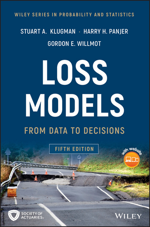
Loss Models (eBook)

From Data to Decisions

Stuart A. Klugman, Harry H. Panjer, Gordon E. Willmot (Autoren)

eBook Download: EPUB

2019 | 5. Auflage
John Wiley & Sons (Verlag)
978-1-119-52375-8 (ISBN)

Infos

A guide that provides in-depth coverage of modeling techniques used throughout many branches of actuarial science, revised and updated

Now in its fifth edition, Loss Models: From Data to Decisions puts the focus on material tested in the Society of Actuaries (SOA) newly revised Exams STAM (Short-Term Actuarial Mathematics) and LTAM (Long-Term Actuarial Mathematics). Updated to reflect these exam changes, this vital resource offers actuaries, and those aspiring to the profession, a practical approach to the concepts and techniques needed to succeed in the profession. The techniques are also valuable for anyone who uses loss data to build models for assessing risks of any kind.

Loss Models contains a wealth of examples that highlight the real-world applications of the concepts presented, and puts the emphasis on calculations and spreadsheet implementation. With a focus on the loss process, the book reviews the essential quantitative techniques such as random variables, basic distributional quantities, and the recursive method, and discusses techniques for classifying and creating distributions. Parametric, non-parametric, and Bayesian estimation methods are thoroughly covered. In addition, the authors offer practical advice for choosing an appropriate model. This important text:

•    Presents a revised and updated edition of the classic guide for actuaries that aligns with newly introduced Exams STAM and LTAM

•    Contains a wealth of exercises taken from previous exams

•    Includes fresh and additional content related to the material required by the Society of Actuaries (SOA) and the Canadian Institute of Actuaries (CIA)

•    Offers a solutions manual available for further insight, and all the data sets and supplemental material are posted on a companion site

Written for students and aspiring actuaries who are preparing to take the SOA examinations, Loss Models offers an essential guide to the concepts and techniques of actuarial science. 

STUART A. KLUGMAN, PHD, FSA, CERA, is Staff Fellow (Education) at the Society of Actuaries (SOA) and Principal Financial Group Distinguished Professor Emeritus of Actuarial Science at Drake University. He has served as SOA vice president.

HARRY H. PANJER, PHD, FSA, FCIA, CERA, HonFIA, is Distinguished Professor Emeritus in the Department of Statistics and Actuarial Science at the University of Waterloo, Canada. He has served as CIA president and as SOA president.

GORDON E. WILLMOT, PHD, FSA, FCIA, is Munich Re Chair in Insurance and Professor in the Department of Statistics and Actuarial Science at the University of Waterloo, Canada.

Textauszug

1
Modeling

1.1 The Model-Based Approach

The model-based approach should be considered in the context of the objectives of any given problem. Many problems in actuarial science involve the building of a mathematical model that can be used to forecast or predict insurance costs in the future.

A model is a simplified mathematical description that is constructed based on the knowledge and experience of the actuary combined with data from the past. The data guide the actuary in selecting the form of the model as well as in calibrating unknown quantities, usually called parameters. The model provides a balance between simplicity and conformity to the available data.

The simplicity is measured in terms of such things as the number of unknown parameters (the fewer the simpler); the conformity to data is measured in terms of the discrepancy between the data and the model. Model selection is based on a balance between the two criteria, namely, fit and simplicity.

1.1.1 The Modeling Process

The modeling process is illustrated in Figure 1.1, which describes the following six stages:

1. Stage 1 One or more models are selected based on the analyst's prior knowledge and experience, and possibly on the nature and form of the available data. For example, in studies of mortality, models may contain covariate information such as age, sex, duration, policy type, medical information, and lifestyle variables. In studies of the size of an insurance loss, a statistical distribution (e.g. lognormal, gamma, or Weibull) may be chosen.
2. Stage 2 The model is calibrated based on the available data. In mortality studies, these data may be information on a set of life insurance policies. In studies of property claims, the data may be information about each of a set of actual insurance losses paid under a set of property insurance policies.
3. Stage 3 The fitted model is validated to determine if it adequately conforms to the data. Various diagnostic tests can be used. These may be well-known statistical tests, such as the chi-square goodness-of-fit test or the Kolmogorov–Smirnov test, or may be more qualitative in nature. The choice of test may relate directly to the ultimate purpose of the modeling exercise. In insurance-related studies, the total loss given by the fitted model is often required to equal the total loss actually experienced in the data. In insurance practice, this is often referred to as unbiasedness of a model.
4. Stage 4 An opportunity is provided to consider other possible models. This is particularly useful if Stage 3 revealed that all models were inadequate. It is also possible that more than one valid model will be under consideration at this stage.
5. Stage 5 All valid models considered in Stages 1–4 are compared, using some criteria to select between them. This may be done by using the test results previously obtained or it may be done by using another criterion. Once a winner is selected, the losers may be retained for sensitivity analyses.
6. Stage 6 Finally, the selected model is adapted for application to the future. This could involve adjustment of parameters to reflect anticipated inflation from the time the data were collected to the period of time to which the model will be applied.

Figure 1.1 The modeling process.

As new data are collected or the environment changes, the six stages will need to be repeated to improve the model.

In recent years, actuaries have become much more involved in “big data” problems. Massive amounts of data bring with them challenges that require adaptation of the steps outlined above. Extra care must be taken to avoid building overly complex models that match the data but perform less well when used to forecast future observations. Techniques such as hold-out samples and cross-validation are employed to addresses such issues. These topics are beyond the scope of this book. There are numerous references available, among them [61].

1.1.2 The Modeling Advantage

Determination of the advantages of using models requires us to consider the alternative: decision-making based strictly upon empirical evidence. The empirical approach assumes that the future can be expected to be exactly like a sample from the past, perhaps adjusted for trends such as inflation. Consider Example 1.1.

Example 1.1

A portfolio of group life insurance certificates consists of 1,000 employees of various ages and death benefits. Over the past five years, 14 employees died and received a total of 580,000 in benefits (adjusted for inflation because the plan relates benefits to salary). Determine the empirical estimate of next year's expected benefit payment.

The empirical estimate for next year is then 116,000 (one-fifth of the total), which would need to be further adjusted for benefit increases. The danger, of course, is that it is unlikely that the experience of the past five years will accurately reflect the future of this portfolio, as there can be considerable fluctuation in such short-term results.

It seems much more reasonable to build a model, in this case a mortality table. This table would be based on the experience of many lives, not just the 1,000 in our group. With this model, not only can we estimate the expected payment for next year, but we can also measure the risk involved by calculating the standard deviation of payments or, perhaps, various percentiles from the distribution of payments. This is precisely the problem covered in texts such as [25] and [28].

This approach was codified by the Society of Actuaries Committee on Actuarial Principles. In the publication “Principles of Actuarial Science” [114, p. 571], Principle 3.1 states that “Actuarial risks can be stochastically modeled based on assumptions regarding the probabilities that will apply to the actuarial risk variables in the future, including assumptions regarding the future environment.” The actuarial risk variables referred to are occurrence, timing, and severity – that is, the chances of a claim event, the time at which the event occurs if it does, and the cost of settling the claim.

1.2 The Organization of This Book

This text takes us through the modeling process but not in the order presented in Section 1.1. There is a difference between how models are best applied and how they are best learned. In this text, we first learn about the models and how to use them, and then we learn how to determine which model to use, because it is difficult to select models in a vacuum. Unless the analyst has a thorough knowledge of the set of available models, it is difficult to narrow the choice to the ones worth considering. With that in mind, the organization of the text is as follows:

1. Review of probability – Almost by definition, contingent events imply probability models. Chapters 2 and 3 review random variables and some of the basic calculations that may be done with such models, including moments and percentiles.
2. Understanding probability distributions – When selecting a probability model, the analyst should possess a reasonably large collection of such models. In addition, in order to make a good a priori model choice, the characteristics of these models should be available. In Chapters 4–7, various distributional models are introduced and their characteristics explored. This includes both continuous and discrete distributions.
3. Coverage modifications – Insurance contracts often do not provide full payment. For example, there may be a deductible (e.g. the insurance policy does not pay the first $250) or a limit (e.g. the insurance policy does not pay more than $10,000 for any one loss event). Such modifications alter the probability distribution and affect related calculations such as moments. Chapter 8 shows how this is done.
4. Aggregate losses – To this point, the models are either for the amount of a single payment or for the number of payments. Of interest when modeling a portfolio, line of business, or entire company is the total amount paid. A model that combines the probabilities concerning the number of payments and the amounts of each payment is called an aggregate loss model. Calculations for such models are covered in Chapter 9.
5. Introduction to mathematical statistics – Because most of the models being considered are probability models, techniques of mathematical statistics are needed to estimate model specifications and make choices. While Chapters 10 and 11 are not a replacement for a thorough text or course in mathematical statistics, they do contain the essential items that are needed later in this book. Chapter 12 covers estimation techniques for counting distributions, as they are of particular importance in actuarial work.
6. Bayesian methods – An alternative to the frequentist approach to estimation is presented in Chapter 13. This brief introduction introduces the basic concepts of Bayesian methods.
7. Construction of empirical models – Sometimes it is appropriate to work with the empirical distribution of the data. This may be because the volume of data is sufficient or because a good portrait of the data is needed. Chapter 14 covers empirical models for the simple case of straightforward data, adjustments for truncated and censored data, and modifications suitable for large data sets, particularly those...

Produkt-Details

• Erscheint lt. Verlag: 4.4.2019
• Reihe/Serie: Wiley Series in Probability and Statistics
• Reihe/Serie: Wiley Series in Probability and Statistics
• Reihe/Serie: Wiley Series in Probability and Statistics
• Sprache: englisch
• Themenwelt: Mathematik / Informatik ► Mathematik ► Statistik
• Themenwelt: Mathematik / Informatik ► Mathematik ► Wahrscheinlichkeit / Kombinatorik
• Themenwelt: Recht / Steuern ► Wirtschaftsrecht
• Themenwelt: Betriebswirtschaft / Management ► Spezielle Betriebswirtschaftslehre ► Versicherungsbetriebslehre
• Schlagworte: analysis of actuary models • analysis of mathematical models for actuaries • applications of models for actuaries • Bayesian estimation methods • Business & Finance • calculations for actuaries • concepts of actuarial models • construct actuary models • creating spread sheet for actuaries • design actuary models • examples of actuary models • examples of estimation methods for actuaries • Finance & Investments • Finanzmathematik • Finanz- u. Anlagewesen • Finanz- u. Wirtschaftsstatistik • <p>Guide to Loss Models • Mathematics • Mathematik • Mathematik in Wirtschaft u. Finanzwesen • modelling techniques in actuarial science • newest material for actuary exam • non-parametric estimation methods • parametric estimation methods • practical guide to concepts of actuarial models • quantitative techniques for actuaries • resource to loss models • risk models for actuaries </p> • society of actuaries exam C • Statistics • Statistics for Finance, Business & Economics • Statistik • text on loss models • Understanding loss models • Wirtschaftsstatistik
• ISBN-10: 1-119-52375-3 / 1119523753
• ISBN-13: 978-1-119-52375-8 / 9781119523758