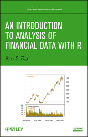
An Introduction to Analysis of Financial Data with R (eBook)
John Wiley & Sons (Verlag)
978-1-119-01346-4 (ISBN)
A complete set of statistical tools for beginning financial analysts from a leading authority
Written by one of the leading experts on the topic, An Introduction to Analysis of Financial Data with R explores basic concepts of visualization of financial data. Through a fundamental balance between theory and applications, the book supplies readers with an accessible approach to financial econometric models and their applications to real-world empirical research.
The author supplies a hands-on introduction to the analysis of financial data using the freely available R software package and case studies to illustrate actual implementations of the discussed methods. The book begins with the basics of financial data, discussing their summary statistics and related visualization methods. Subsequent chapters explore basic time series analysis and simple econometric models for business, finance, and economics as well as related topics including:
- Linear time series analysis, with coverage of exponential smoothing for forecasting and methods for model comparison
- Different approaches to calculating asset volatility and various volatility models
- High-frequency financial data and simple models for price changes, trading intensity, and realized volatility
- Quantitative methods for risk management, including value at risk and conditional value at risk
- Econometric and statistical methods for risk assessment based on extreme value theory and quantile regression
Throughout the book, the visual nature of the topic is showcased through graphical representations in R, and two detailed case studies demonstrate the relevance of statistics in finance. A related website features additional data sets and R scripts so readers can create their own simulations and test their comprehension of the presented techniques.
An Introduction to Analysis of Financial Data with R is an excellent book for introductory courses on time series and business statistics at the upper-undergraduate and graduate level. The book is also an excellent resource for researchers and practitioners in the fields of business, finance, and economics who would like to enhance their understanding of financial data and today's financial markets.
RUEY S. TSAY, PhD, is H.G.B. Alexander Professor of Econometrics and Statistics at The University of Chicago Booth School of Business. Dr. Tsay has written over 100 published articles in the areas of business and economic forecasting, data analysis, risk management, and process control. A Fellow of the American Statistical Association, the Institute of Mathematical Statistics, and Academia Sinica, Dr. Tsay is author of Analysis of Financial Time Series, Third Edition and coauthor of A Course in Time Series Analysis.
RUEY S. TSAY, PhD, is H.G.B. Alexander Professor of Econometrics and Statistics at The University of Chicago Booth School of Business. Dr. Tsay has written over 100 published articles in the areas of business and economic forecasting, data analysis, risk management, and process control. A Fellow of the American Statistical Association, the Institute of Mathematical Statistics, and Academia Sinica, Dr. Tsay is author of Analysis of Financial Time Series, Third Edition and coauthor of A Course in Time Series Analysis.
"I found this book highly informative and interesting to
read. The proper mix of theory and hands-on programming examples
makes it recommended reading for both R programmers interested in
finance and financial analysts with a basic programming background.
Well written and following a clear and defined logical layout, the
author has written a current reference text on using a powerful
open-source programming language for typical financial
analysis." (Computing Reviews, 25 March
2014)
"All in all, this book is a good and useful introduction
to financial time series with many real-world examples. It is
suitable for use both as a textbook and for self-study, with
exercises provided at the end of each chapter."
(International Statistical Review, 14 June 2013)
1
FINANCIAL DATA AND THEIR PROPERTIES
The importance of quantitative methods in business and finance has increased substantially in recent years because we are in a data-rich environment and the economies and financial markets are more integrated than ever before. Data are collected systematically for thousands of variables in many countries and at a finer timescale. Computing facilities and statistical packages for analyzing complicated and high dimensional financial data are now widely available. As a matter of fact, with an internet connection, one can easily download financial data from open sources within a software package such as R. All of these good features and capabilities are free and widely accessible.
The objective of this book is to provide basic knowledge of financial time series, introduce statistical tools useful for analyzing financial data, and gain experience in financial applications of various econometric methods. We begin with the basic concepts of financial data to be analyzed throughout the book. The software R is introduced via examples. We also discuss different ways to visualize financial data in R. Chapter 2 reviews basic concepts of linear time series analysis such as stationarity and autocorrelation function, introduces simple linear models for handling serial dependence of the data, and discusses regression models with time series errors, seasonality, unit-root nonstationarity, and long-memory processes. The chapter also considers exponential smoothing for forecasting and methods for model comparison. Chapter 3 considers some applications of the models introduced in Chapter 2 in the form of case studies. The goal is to help readers understand better data analysis, empirical modeling, and making inference. It also points out the limitations of linear time series models in long-term prediction. Chapter 4 focuses on modeling conditional heteroscedasticity (i.e., the conditional variance of an asset return). It introduces various econometric models for describing the evolution of asset volatility over time. The chapter also discusses alternative methods to volatility modeling, including use of daily high and low prices of an asset. In Chapter 5, we demonstrate some applications of volatility models using, again, some case studies. All steps for building volatility models are given, and the merits and weaknesses of various volatility models are discussed, including the connection to diffusion limit of continuous time models. Chapter 6 is concerned with analysis of high frequency financial data. It starts with special characteristics of high frequency data and gives models and methods that can be used to analyze such data. It shows that nonsynchronous trading and bid-ask bounce can introduce serial correlations in a stock return. It also studies the dynamic of time duration between trades and some econometric models for analyzing transaction data. In particular, we discuss the use of logistic linear regression and probit models to study the stock price movements in consecutive trades. Finally, the chapter studies the realized volatility using intraday log returns. Chapter 7 discusses risk measures of a financial position and their use in risk management. It introduces value at risk and conditional value at risk to quantify the risk of a financial position within a holding period. It also provides various methods for calculating risk measures for a financial position, including RiskMetrics, econometric modeling, extreme value theory, quantile regression, and peaks over thresholds.
The book places great emphasis on application and empirical data analysis. Every chapter contains real examples, and, in many occasions, empirical characteristics of financial time series are used to motivate the development of econometric models. In some cases, simple R scripts are given on the web page for specific analysis. Many real data sets are also used in the exercises of each chapter.
1.1 ASSET RETURNS
Most financial studies involve returns, instead of prices, of assets. Campbell et al. (1997) give two main reasons for using returns. First, for average investors, return of an asset is a complete and scale-free summary of the investment opportunity. Second, return series are easier to handle than price series because the former have more attractive statistical properties. There are, however, several definitions of an asset return.
Let Pt be the price of an asset at time index t. We discuss some definitions of returns that are used throughout the book. Assume for the moment that the asset pays no dividends.
One-Period Simple Return. Holding the asset for one period from date t − 1 to date t would result in a simple gross return
(1.1)
The corresponding one-period simple net return or simple return is
(1.2)
For demonstration, Table 1.1 gives five daily closing prices of Apple stock in December 2011. From the table, the 1-day gross return of holding the stock from December 8 to December 9 is 1 + Rt = 393.62/390.66 ≈ 1.0076 so that the corresponding daily simple return is 0.76%, which is (393.62-390.66)/390.66.
Multiperiod Simple Return. Holding the asset for k periods between dates t − k and t gives a k-period simple gross return
Thus, the k-period simple gross return is just the product of the k one-period simple gross returns involved. This is called a compound return. The k-period simple net return is
To ile daily closing prices of Apple stock of Table 1.1. Since December 2 and 9 are Fridays, the weekly simple gross return of the stock is 1 + Rt [5] = 393.62/389.70 ≈ 1.0101 so that the weekly simple return is 1.01%.
In practice, the actual time interval is important in discussing and comparing returns (e.g., monthly return or annual return). If the time interval is not given, then it is implicitly assumed to be one year. If the asset was held for k years, then the annualized (average) return is defined as
TABLE 1.1. Daily Closing Prices of Apple Stock from December 2 to 9, 2011
This is a geometric mean of the k one-period simple gross returns involved and can be computed by
where exp(x) denotes the exponential function and ln(x) is the natural logarithm of the positive number x. Because it is easier to compute arithmetic average than geometric mean and the one-period returns tend to be small, one can use a first-order Taylor expansion to approximate the annualized return and obtain
Accuracy of the approximation in Equation (1.3) may not be sufficient in some applications, however.
Continuous Compounding. Before introducing continuously compounded return, we discuss the effect of compounding. Assume that the interest rate of a bank deposit is 10% per annum and the initial deposit is $1.00. If the bank pays interest once a year, then the net value of the deposit becomes $1(1+0.1) = $1.1, 1 year later. If the bank pays interest semiannually, the 6-month interest rate is 10%/2 = 5% and the net value is $ 1(1 + 0.1/2)2 = $1.1025 after the first year. In general, if the bank pays interest m times a year, then the interest rate for each payment is 10%/m and the net value of the deposit becomes $1(1 + 0.1/m)m , 1 year later. Table 1.2 gives the results for some commonly used time intervals on a deposit of $1.00 with interest rate of 10% per annum. In particular, the net value approaches $1.1052, which is obtained by exp(0.1) and referred to as the result of continuous compounding. The effect of compounding is clearly seen.
TABLE 1.2. Illustration of the Effects of Compounding: the Time Interval is 1 Year and the Interest Rate is 10% Per Annum
In general, the net asset value A of continuous compounding is
where r is the interest rate per annum, C is the initial capital, and n is the number of years. From Equation (1.4), we have
(1.5)
which is referred to as the present value of an asset that is worth A dollars n years from now, assuming that the continuously compounded interest rate is r per annum.
Continuously Compounded Return. The natural logarithm of the simple gross return of an asset is called the continuously compounded return or log return:
(1.6)
where pt = ln(Pt). Continuously compounded returns rt enjoy some advantages over the simple net returns Rt. First, consider multiperiod returns. We have
Thus, the continuously compounded multiperiod return is simply the sum of continuously compounded one-period returns involved. Second, statistical properties of log returns are more tractable.
To demonstrate, we again consider the daily closing prices of Apple stock of Table 1.1. The daily log return from December 8 to December 9 is rt = log(393.62) − log(390.66) ≈ 0.75% and the weekly log return from December 2 to December 9 is rt [5] = log(393.62) − log(389.70) ≈ 1.00%. One can easily verify that the weekly log return is the sum of the five daily log returns involved.
Portfolio Return. The simple net return of a portfolio consisting of N assets is a weighted average of the simple net returns of the assets involved, where the weight on each...
| Erscheint lt. Verlag | 21.8.2014 |
|---|---|
| Reihe/Serie | Wiley Series in Probability and Statistics |
| Wiley Series in Probability and Statistics | Wiley Series in Probability and Statistics |
| Sprache | englisch |
| Themenwelt | Mathematik / Informatik ► Mathematik ► Statistik |
| Mathematik / Informatik ► Mathematik ► Wahrscheinlichkeit / Kombinatorik | |
| Technik | |
| Wirtschaft ► Betriebswirtschaft / Management ► Finanzierung | |
| Wirtschaft ► Volkswirtschaftslehre ► Ökonometrie | |
| Schlagworte | Finance & Investments • Financial Engineering • Finanztechnik • Finanz- u. Anlagewesen • Finanz- u. Wirtschaftsstatistik • high frequency financial, empirical financial data, financial time series data, financial econometric models, predicting financial data, financial statistics, financial data analysis • Statistics • Statistics for Finance, Business & Economics • Statistik • Time Series • Wirtschaftsstatistik • Zeitreihen |
| ISBN-10 | 1-119-01346-1 / 1119013461 |
| ISBN-13 | 978-1-119-01346-4 / 9781119013464 |
| Informationen gemäß Produktsicherheitsverordnung (GPSR) | |
| Haben Sie eine Frage zum Produkt? |
Kopierschutz: Adobe-DRM
Adobe-DRM ist ein Kopierschutz, der das eBook vor Mißbrauch schützen soll. Dabei wird das eBook bereits beim Download auf Ihre persönliche Adobe-ID autorisiert. Lesen können Sie das eBook dann nur auf den Geräten, welche ebenfalls auf Ihre Adobe-ID registriert sind.
Details zum Adobe-DRM
Dateiformat: EPUB (Electronic Publication)
EPUB ist ein offener Standard für eBooks und eignet sich besonders zur Darstellung von Belletristik und Sachbüchern. Der Fließtext wird dynamisch an die Display- und Schriftgröße angepasst. Auch für mobile Lesegeräte ist EPUB daher gut geeignet.
Systemvoraussetzungen:
PC/Mac: Mit einem PC oder Mac können Sie dieses eBook lesen. Sie benötigen eine
eReader: Dieses eBook kann mit (fast) allen eBook-Readern gelesen werden. Mit dem amazon-Kindle ist es aber nicht kompatibel.
Smartphone/Tablet: Egal ob Apple oder Android, dieses eBook können Sie lesen. Sie benötigen eine
Geräteliste und zusätzliche Hinweise
Buying eBooks from abroad
For tax law reasons we can sell eBooks just within Germany and Switzerland. Regrettably we cannot fulfill eBook-orders from other countries.
aus dem Bereich


