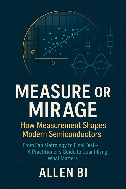
Measure or Mirage (eBook)

How Measurement Shapes Modern Semiconductors

Allen Bi (Autor)

eBook Download: EPUB

2025 | 1. Auflage
168 Seiten
Publishdrive (Verlag)
978-0-00-109045-3 (ISBN)

Infos

Semiconductors run on numbers. From nanometer-scale features to terabit-per-second links, nothing works until it is measured, characterized, and proven. Measure or Mirage is a practitioner's tour-from fab metrology and WAT, through bring-up, reliability, wafer sort, final ATE, and system-level test-showing how measurement turns physics into products. Blending clear explanations with real-world checklists, this book demystifies wave-particle 'probability everywhere,' makes sense of margins, jitter, leakage, and drift, and shows how statistics and test strategy convert raw signals into trusted silicon. Whether you're a student, software/EE new to chips, or a seasoned engineer crossing domains, you'll learn what to measure, why it matters, and how to decide. Written by an industry insider with 10+ years hands-on experience across memory and logic, this is your map for turning theory into yield-one measurement at a time.

 

Author: Allen Bi - Semiconductor engineer with 10+ years in memory test, reliability, and system validation at INTEL.

Textauszug

Part I

Why Measurement Rules Everything

Chapter 1 — Measurability: From Probability to Product

Mantra: If you can’t measure it, you can’t decide it; if you can’t decide it, you can’t ship it.

Semiconductors turn the invisible into the indispensable. We route electrons through structures smaller than wavelengths of light and promise that trillions of devices will behave within tight limits across time, voltage, and temperature. The bridge between quantum-scale uncertainty and production-scale certainty is measurement—not as a one-off act, but as a disciplined system: instruments, methods, sampling, statistics, and decisions. This chapter lays that foundation.

1.1 Why “measurability” comes first

A design intent (“read latency ≤ 12 cycles at 1.1 V, 85 °C”) is a hypothesis. To ship product, we must operationalize that hypothesis as a measurement procedure that any trained engineer can repeat and that will, with known uncertainty, declare pass/fail in realistic variation.

Think of measurability as a contract with the future:

• The what: the quantity of interest (QoI)—e.g., eye height, leakage, VthV_{th}, SN sense margin.

• The how: the method—fixtures, pattern, dwell, filtering, temperature soak, averaging, analysis.

• The error: the uncertainty budget—bias, repeatability, reproducibility, drift, linearity.

• The decision: the rule—guard bands, confidence, Type I/II error, actions on fail.

Key idea: A specification is not a magic number; it is a probabilistic promise conditioned on a measurement definition.

1.2 From wave–particle to yield: probability everywhere

At the microscopic scale, wave–particle duality forces us to speak in distributions, not constants. At the macroscopic scale, huge populations (billions of cells, thousands of wafers) make statistics unavoidable: even if every device were identical, the act of measuring introduces variation.

• Quantum hint: We never observe “the” VthV_{th}; we observe a distribution of VthV_{th} under fixed test conditions.

• Engineering translation: We must summarize behavior via mean, spread, tails, and confidence.

• Business translation: Yield and DPPM are tail integrals of those distributions against decision thresholds.

Specification as probability:
“I_DDQ ≤ 10 µA at 25 °C, 1.1 V” means: when measured by a defined method, the probability of true escapes and overkills under production variation is acceptably low.

1.3 Measurement models and uncertainty budgets

A simple model:

Observed=True+Bias+RandomErrorObserved = True/mathbf{+}Bias/mathbf{+}Random/ Error

• Bias (systematic): fixture offset, ADC calibration, probe contact force, thermal gradients.

• Random error: noise, short-term drift, quantization, environmental fluctuations.

• Linearity: does bias change across the range (e.g., current shunt nonlinearity)?

• Stability: does the system change over time (probe wear, instrument warm-up)?

Uncertainty budget lists contributors (units, distribution, estimate, source) and combines them (RSS for independent components) to a standard uncertainty u. Decisions often use expanded uncertainty U=kuU = ku (coverage factor k≈2 for ~95 % under near-normal conditions).

Practical rule of thumb: If measurement spread is a large fraction of process spread, you will misclassify units. Fix the gauge before tuning the process.

1.4 MSA: Repeatability, Reproducibility, GR&R

A minimal Measurement System Analysis (MSA) answers:

1. Repeatability: How consistent is one operator/instrument on the same unit?

2. Reproducibility: How much extra spread appears across operators/instruments/sites?

3. GR&R: What fraction of total observed variance is due to the gauge?

Let σtotal2=σpart2+σgauge2/sigma_{total}^{2} = /sigma_{part}^{2} + /sigma_{gauge}^{2}

Define %GR&R=σgaugeσtotal×100%/% GR/& R = /frac{/sigma_{gauge}}{/sigma_{total}} /times 100/%

• Interpretation (common practice):

  • < 10 %: good; 10–30 %: marginal (use with caution/Improve); > 30 %: poor (fix gauge or method).

• Linearity & bias: test artifacts at multiple setpoints; compare to a traceable standard.

• Stability: remeasure control parts over days/weeks; watch for drift.

Sidebar — Fast MSA for busy labs

• Choose 10–12 parts spanning your range (e.g., “fast/type/slow” dies).

• 3 operators × 2 repeats each.

• Randomize run order, re-probe after thermal soak.

• Use ANOVA GR&R, plot components of variance.

• If %GR&R too high, check probe planarity, contact resistance, instrument bandwidth, and settle-time.

1.5 Sampling: lots, wafers, dies, and the power to see differences

You cannot measure “everything.” You must sample wisely to detect meaningful effects.

1.5.1 Stratified sampling

When populations are naturally grouped (lots, wafers, corners, banks), sample within each stratum to reduce variance and prevent confounding (e.g., a single bad wafer dominating your estimate).

1.5.2 How many samples?

For estimating a mean with margin of error EEE at 95 % confidence:

n≈(1.96σE)2n/ /approx / {(/frac{1.96/sigma}{E})}^{2}

For a proportion (e.g., fail rate p):

n≈1.962p(1−p)E2n/ /approx / /frac{{1.96}^{2}p(1 - p)}{E^{2}}

When σ and p are unknown, pilot first. For detection of a shift Δ with power 1−βat size α, the two-sample normal approximation:

n≈2(z1−α2+z1−βΔσ)2n/ /approx / {2/ (/frac{z_{1 - /frac{/alpha}{2}} + z_{1 - /beta}}{/frac{/mathrm{/Delta}}{/sigma}})}^{2}

Engineering reading: Big effects need few samples; tiny effects require many. Spend samples where decisions change.

1.6 Hypotheses, errors, and guard bands

Every pass/fail is a hypothesis test.

• Type I error (α): shipping a bad unit (escape).

• Type II error (β): killing a good unit (overkill).

• Power (1 − β): probability to catch a real defect.

Guard bands shift your decision threshold to compensate for measurement uncertainty and protect against escapes. If the spec is SSS and measurement has expanded uncertainty UUU:

• For an upper spec (e.g., leakage ≤ S), decide pass only if x≤S−g, where g reflects U and your tolerated α.

• For a lower spec, mirror accordingly.

Operating Characteristic (OC) curve visualizes escape/overkill vs. true value across thresholds—great for tuning screening vs. yield.

1.7 “Margin” as the universal currency

Whether it’s DRAM sense margin, PLL jitter margin, or DDR timing margin, margin = distance from failure under defined conditions.

• Static margin: measured at a snapshot (e.g., eye height at 25 °C).

• Dynamic margin: worst-case across sweeps (V/T/frequency/pattern).

• Spend vs. save: You can spend margin to gain performance/power, but you cannot spend a margin you didn’t measure.

Working definition:

Margin=minconditions(SpecLimit−MeasuredQuantity)Margin = /min_{conditions}{(Spec/ Limit - Measured/ Quantity)}

with sign and direction chosen so positive = safe.

Tie margin to use cases: idle/active, burst/steady, corner lots, early life vs. aged. Measuring only at “typ/room” is a plan to be surprised.

1.8 Visualizing distributions that decide money

Pick plots that answer decisions, not decorate reports.

• CDF: best for tail probabilities (yield, DPPM).

• Box & violin: quick spread/median and multimodality hints.

• QQ plot: check normality—a straight line is your friend.

• Control charts (SPC): time-ordered data with limits reveals drift/shifts.

• Scatter + faceting: separate wafers/lots/corners in the same figure; avoid mixing conditions.

• Heatmaps: wafer maps and 2D arrays (e.g., sense margin across banks) highlights spatial signatures.

Always annotate N, conditions, and units on plots. A beautiful unlabeled plot is a rumor.

1.9 Case vignette: a tail that sank yield

A team measured DDR read setup margin at room temperature and saw a comfortable average with narrow spread. Final test later reported intermittent fails at high...

Produkt-Details

• Erscheint lt. Verlag: 14.10.2025
• Sprache: englisch
• Themenwelt: Technik ► Elektrotechnik / Energietechnik
• ISBN-10: 0-00-109045-3 / 0001090453
• ISBN-13: 978-0-00-109045-3 / 9780001090453