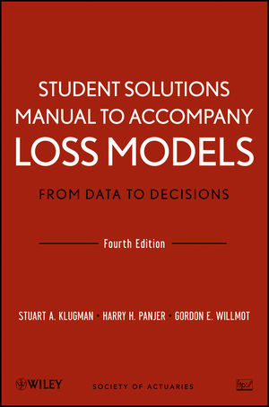
Loss Models: From Data to Decisions, 4e Student Solutions Manual (eBook)

Stuart A. Klugman, Harry H. Panjer, Gordon E. Willmot (Autoren)

eBook Download: EPUB

2014 | 4. Auflage
John Wiley & Sons (Verlag)
978-1-118-47202-6 (ISBN)

Infos

Student Solutions Manual to Accompany Loss Models: From Data to Decisions, Fourth Edition. This volume is organised around the principle that much of actuarial science consists of the construction and analysis of mathematical models which describe the process by which funds flow into and out of an insurance system.

Autor

STUART A. KLUGMAN, PhD, is Principal Financial Group Distinguished Professor of Actuarial Science at Drake University. A Fellow of the Society of Actuaries, Dr. Klugman was vice president of the SOA from 2001 to 2003. HARRY H. PANJER, PhD, is Professor Emeritus in the Department of Statistics and Actuarial Science at the University of Waterloo, Canada. Past president of both the Canadian Institute of Actuaries and the Society of Actuaries, Dr. Panjer has published numerous articles on risk modeling in the fields of finance and actuarial science.

Inhalt

Introduction--A Model-Based Approach to Actuarial Science.

Loss Distributions--Models for the Amount of a Single Payment.

Frequency Distributions--Models for the Number of Payments.

Aggregate Loss Models.

Credibility Theory.

Long-Term Models.

Appendices.

References.

Index.

Textauszug

CHAPTER 3

CHAPTER 3 SOLUTIONS

3.1 SECTION 3.1

3.1

3.2 For Model 1, σ2 = 3,333.33 – 502 = 833.33, σ = 28.8675.

For Model 2, σ2 = 4,000,000 – 1,0002 = 3,000,000, σ = 1,732.05. and are both infinite so the skewness and kurtosis are not defined.

For Model 3, σ2 = 2.25 – .932 = 1.3851, σ = 1.1769.

For Model 4, σ2 = 6,000,000,000 – 30,0002 = 5,100,000,000, σ = 71,414.

For Model 5, σ2 = 2,395.83 – 43.752 = 481.77, σ = 21.95.

3.3 The Standard deviation is the mean times the coefficient, of Variation, or 4, and so the variance is 16. From (3.3) the second raw moment is 16 + 22 = 20. The third central moment is (using Exercise 3.1) 136 – 3(20)(2) + 2(2)3 = 32. The skewness is the third central moment divided by the cube of the Standard deviation, or 32/43 = 1/2.

3.4 For a gamma distribution the mean is αθ. The second raw moment is α(α + 1)θ2, and so the variance is αθ2. The coefficient of Variation is /αθ = α–1/2 = 1. Therefore α = 1. The third raw moment is α(α + 1)(α + 2)θ3 = 6θ3. From Exercise 3.1, the third central moment is 6θ3 – 3(2θ2)θ + 2θ3 = 2θ3 and the skewness is 2θ3/(θ2)3/2 = 2.

3.5 For Model 1,

For Model 2,

For Model 3,

For Model 4,

The functions are straight lines for Models 1, 2, and 4. Model 1 has negative slope, Model 2 has positive slope, and Model 4 is horizontal.

3.6 For a uniform distribution on the interval from 0 to w, the density function is f(x) = 1/w. The mean residual life is

The equation becomes

with a solution of w = 108.

3.7 From the definition,

3.8

3.9 For Model 1, from (3.8),

and from (3.10),

From (3.9),

For Model 2, from (3.8),

and from (3.10),

From (3.9),

For Model 3, from (3.8),

and from (3.10),

For Model 4, from (3.8),

and from (3.10),

3.10 For a discrete distribution (which all empirical distributions are), the mean residual life function is

When d is equal to a possible value of X, the function cannot be continuous because there is jump in the denominator but not in the numerator. For an exponential distribution, argue as in Exercise 3.7 to see that it is constant. For the Pareto distribution,

which is increasing in d. Only the second statement is true.

3.11 Applying the formula from the solution to Exercise 3.10 gives

which cannot be correct. Recall that the numerator of the mean residual life is E(X)–E(X d). However, when α ≤ 1, the expected value is infinite and so is the mean residual life.

3.12 The right truncated variable is defined as Y = X given that X ≤ u. When X > u, this variable is not defined. The kth moment is

3.13 This is a single parameter Pareto distribution with parameters α = 2.5 and θ = 1. The moments are μ1 = 2.5/1.5 = 5/3 and μ2 = 2.5/.5 – (5/3)2 = 20/9. The coefficient of Variation is /(5/3) = 0.89443.

3.14 μ = 0.05(100) + 0.2(200) + 0.5(300) + 0.2(400) + 0.05(500) = 300.
σ2 = 0.05(–200)2 + 0.2(–100)2 + 0.5(0)2 + 0.2(100)2 + 0.05(200)2 = 8,000.
μ3 = 0.05(–200)3 + 0.2(–100)3 + 0.5(0)3 + 0.2(100)3 + 0.05(200)3 = 0.
μ4 = 0.05(–200)4+0.2(–100)4+0.5(0)4+0.2(100)4+0.05(200)4 = 200,000,000.

Skewness is = γ1 = μ3/σ3 = 0. Kurtosis is γ2 = μ4/σ4 = 200,000,000/8,0002 = 3.125.

3.15 The Pareto mean residual life function is

and so eX (2θ)/eX(θ) = (2θ + θ)/(θ + θ) = 1.5.

3.16 Sample mean: 0.2(400) + 0.7(800) + 0.1(1,600) = 800. Sample variance: 0.2(–400)2 + 0.7(0)2 + 0.1(800)2 = 96,000. Sample third central moment: 0.2(–400)3 + 0.7(0)3 + 0.1 (800)3 = 38,400,000. Skewness coefficient: 38,400,000/96,0001.5 = 1.29.

3.2 SECTION 3.2

3.17 The pdf is f(x) = 2x–3, x ≥ 1. The mean is 2x–2dx = 2. The median is the solution to .5 = F(x) = 1 – x–2, which is 1.4142. The mode is the value where the pdf is highest. Because the pdf is strictly decreasing, the mode is at its smallest value, 1.

3.18 For Model 2, solve and so πp = 2,000[(1 – p)–1/3 – 1] and the requested percentiles are 519.84 and 1419.95.

For Model 4, the distribution function jumps from 0 to 0.7 at zero and so π0.5 = 0. For percentile above 70, solve p = 1 – 0.3e–0.00001πp, and so πp = –100,000 ln[(1 – p)/0.3] and π0.8 = 40,546.51.

For Model 5, the distribution function has two specifications. From x = 0 to x = 50 it rises from 0.0 to 0.5, and so for percentiles at 50 or below, the equation to solve is p = 0.01πp for πp = 100p. For 50 < x ≤ 75, the distribution function rises from 0.5 to 1.0, and so for percentiles from 50 to 100 the equation to solve is p = 0.02πp – 0.5 for πp = 50p + 25. The requested percentiles are 50 and 65.

3.19 The two percentiles imply

Rearranging the equations and taking their ratio yield

Taking logarithms of both sides gives ln 9 = α ln 3 for α = ln 9/ln 3 = 2.

3.20 The two percentiles imply

Subtracting and then taking logarithms of both sides give

Dividing the second equation by the first gives

Finally, taking logarithms of both sides gives τ ln 100 = ln[ln 0.25/ln 0.75] for τ = 0.3415.

3.3 SECTION 3.3

3.21 The sum has a gamma distribution with parameters α = 16 and θ = 250. Then, Pr(S16 > 6,000) = 1 – Γ(16; 6,000/250) = 1 – Γ(16;24). From the Central Limit Theorem, the sum has an approximate normal distribution with mean αθ = 4,000 and variance αθ2 = 1,000,000 for a Standard deviation of 1000. The probability of exceeding 6,000 is 1 – Φ[(6,000 – 4,000)/1,000] = 1 – Φ(2) = 0.0228.

3.22 A single claim has mean 8,000/(5/3) = 4,800 and variance

The sum of 100 claims has mean 480,000 and variance 9,216,000,000, which is a Standard deviation of 96,000. The probability of exceeding 600,000 is approximately

3.23 The mean of the gamma distribution is 5(1,000) = 5,000 and the variance is 5(1,000)2 = 5,000,000. For 100 independent claims, the mean is 500,000 and the variance is 500,000,000 for a Standard deviation of 22,360.68. The probability of total claims exceeding 525,000 is

3.24 The sum of 2,500 contracts has an approximate normal distribution with mean 2,500(1,300) = 3,250,000 and Standard deviation (400) = 20,000. The answer is Pr(X > 3,282,500) Pr[Z > (3,282,500 – 3,250,000)/20,000] = Pr(Z > 1.625) = 0.052.

3.4 SECTION 3.4

3.25 While the Weibull distribution has all positive moments, for the inverse Weibull moments exist only for k < τ. Thus by this criterion, the inverse Weibull distribution has a heavier tail. With regard to the ratio of density functions, it is (with the inverse Weibull in the numerator and marking its Parameters with asterisks)

The logarithm is

The middle term goes to zero, so the issue is the limit of (x/θ)τ – (τ + τ*) ln x, which is clearly infinite. With regard to the hazard rate, for the Weibull distribution we have

Figure 3.1 Tails of a Weibull and inverse Weibull distribution.

which is clearly increasing when τ > 1, constant when τ = 1, and decreasing when τ < 1. For the inverse Weibull,

The derivative of the denominator is

and the limiting value of this expression is θτ > 0. Therefore, in the limit, the denominator is increasing and thus the hazard rate is decreasing.

Figure 3.1 displays a portion of the density function for Weibull (τ = 3, θ = 10) and inverse Weibull (τ = 4.4744, θ = 7.4934) distributions with the same mean and variance. The...

Produkt-Details

• Erscheint lt. Verlag: 21.8.2014
• Reihe/Serie: Wiley Series in Probability and Statistics
• Reihe/Serie: Wiley Series in Probability and Statistics
• Reihe/Serie: Wiley Series in Probability and Statistics
• Sprache: englisch
• Themenwelt: Mathematik / Informatik ► Mathematik ► Statistik
• Themenwelt: Mathematik / Informatik ► Mathematik ► Wahrscheinlichkeit / Kombinatorik
• Themenwelt: Technik
• Schlagworte: accompany • Actuarial • Book • Branches • Business & Finance • Coverage • edition quot • exceptional • Finance & Investments • Finanz- u. Anlagewesen • Finanz- u. Wirtschaftsstatistik • high standard • indepth • Loss • many • Mathematics • Mathematik • Mathematik in Wirtschaft u. Finanzwesen • Modelling • Models • Science • selection • Solutions Manual • Statistics • Statistics for Finance, Business & Economics • Statistik • Student • student solutions manual • techniques • Third • throughout • Wirtschaftsstatistik
• ISBN-10: 1-118-47202-0 / 1118472020
• ISBN-13: 978-1-118-47202-6 / 9781118472026