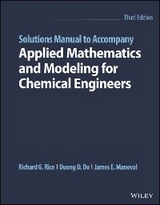
Solutions Manual to Accompany Applied Mathematics and Modeling for Chemical Engineers (eBook)

Richard G. Rice, Duong D. Do, James E. Maneval (Autoren)

eBook Download: EPUB

2023 | 3. Auflage
608 Seiten
Wiley (Verlag)
9781119833925 (ISBN)

Infos

This book is a Solutions Manual to accompany Applied Mathematics and Modeling for Chemical Engineers, Third Edition. There are many examples provided as homework in the original text and the solution manual provides detailed solutions of many of these problems that are in the parent book Applied Mathematics and Modeling for Chemical Engineers, Third Edition.

Richard G. Rice, PhD, is Emeritus Professor (LSU) and widely published in chemical separations and two-phase flow.

Duong D. Do, PhD, is University Professor (University of Queensland, Australia) and is well-known in the area of adsorption science having published two books on the subject.

James E. Maneval, PhD, is an Assistant Professor in the Department of Chemical Engineering at Bucknell University specializing in teaching Applied Mathematics.

Inhalt

1 Formulation of Physicochemical Problems 1

2 Modelling with Linear Algebra and Matrices 21

3 Solution Techniques for Models Yielding Ordinary Differential Equations 71

4 Series Solution Methods and Special Functions 149

5 Integral Functions 181

6 Staged-Process Models: The Calculus of Finite Differences 199

7 Probability and Statistical Modelling 215

8 Approximate Solution Methods for ODE: Perturbation Methods 257

9 Numerical Solution Methods (Initial Value Problems) 305

10 Approximate Methods for Boundary Value Problems: Weighted Residuals 329

11 Introduction to Complex Variables and Laplace Transforms 389

12 Solution Techniques for Models Producing PDEs 417

13 Transform Methods for Linear PDEs 503

14 Approximate and Numerical Solution Methods for PDEs 545

Textauszug

CHAPTER 1
Formulation of Physicochemical Problems

Problem 1.1

Length Required for Cooling Coil

Model 1 – Plug Flow, in section 1.2 applies:

The heat transfer coefficient is obtained from the correlation:

(1.1.1)

where

(1.1.2)

Substitution in Eq. 1.17 (in the text), with T(z) = TL, gives:

(1.1.3)

Solving the above equation for L, we get

(1.1.4)

Problem 1.2

Cooling of Fluids in Tube Flow: Locally Varying h

Model 1 (Section 1.2) applies up to equation 1.8:

(1.2.1)

Substitution of h for gives:

(1.2.2)

Lumping parameters and changing the dependent variable, we get:

(1.2.3)

where:

(1.2.4)

Separation of variables and integration using the boundary condition at z = 0

(1.2.5)

yields:

(1.2.6)

Problem 1.3

Dissolution of Benzoic Acid

Part (a):

Carrying out material balance around the shell at x with a thickness of Δx gives:

(1.3.1)

where

(1.3.2)

Dividing Eq. (1.3.1) by πDΔx gives:

(1.3.3)

Taking the limit as Δx → 0, we get:

(1.3.4)

Part (b):

Defining θ = C − C* and substituting into Eq. (1.3.4), we obtain:

(1.3.5)

Separating the variables and integrating gives:

(1.3.6)

Part (c):

Using the boundary condition at x = 0, θ = −C*, gives

Thus, the final solution for C(x) is:

(1.3.7)

Part (d):

The concentration of benzoic acid leaving the tube at x = L is:

(1.3.8)

The total flow rate through the tube is:

(1.3.9a)

The rate of benzoic acid leaving the tube is:

(1.3.9b)

The weight change of the tube is:

(1.3.9c)

Substituting QT, QB and C(L) in the expression for ΔW, we get:

(1.3.10)

Part (e):

Rearranging Eq. (1.3.10), we get:

(1.3.11)

Approximation of the exponential term:

(1.3.12)

Substitution the above equation into Eq. (1.3.11), rearrangement and simplification gives:

(1.3.13)

Part (f):

Assumptions of the model are:

1. plug flow,
2. only resistance to dissolution of benzoic acid is due to liquid phase film resistance,
3. no axial or radial diffusion,
4. perfect radial mixing, and
5. constant wall diameter.

The maximum error can be estimated by the following equation (absolute value assures that all errors are additives, hence maximum errors):

(1.3.14)

where:

(1.3.15a)

(1.3.15b)

(1.3.15c)

Substitute the values of the partial derivatives using the previous equations and the errors, εΔW, εΔt and εD, from the experimental data, and simplifying:

(1.3.16)

Problem 1.4

Lumped Thermal Model for Thermocouple

Heat balance equation is

(1.4.1)

where

(1.4.2a)

(1.4.2b)

Substituting Eqs. (1.4.2) into Eq. (1.4.1), we get:

(1.4.3)

Part (b):

Defining θ = Tf − T and substituting into Eq. (1.4.3), we have:

(1.4.4)

where:

(1.4.5)

Part (c):

Separating variables and integrating Eq. (1.4.4) with the boundary condition T(0) = T0, we get:

(1.4.6)

Multiplying both sides by −1, adding 1 to each side, and rearranging, we obtain:

(1.4.7)

Evaluating for t = τ, (T0 − T)(T0 − Tf) = 0.63, therefore:

(1.4.8)

Problem 1.5

Distributed Thermal Model for Thermocouple

Heat Balance around the shell at r with a thickness of Δr is:

(1.5.1)

where:

(1.5.2a)

(1.5.2b)

Substituting Q, dividing throughout by 4πΔr and taking the limits as Δr → 0, we get:

(1.5.3)

Substituting qr from Eq. (1.5.2a) into the above equation, and rearranging, we get:

(1.5.4)

Part (b):

Heat balance at the surface of the sphere:

Heat Flux within Sphere by Conduction = Heat Flux to fluid by convection

Mathematically this continuity of heat flux is:

(1.5.5)

where:

(1.5.6a)

(1.5.6b)

Substituting qcond and qconv into Eq. (1.5.5), we get the boundary condition at r = R:

(1.5.7)

Problem 1.6

Modelling of Piston with Restraining Spring

Force Balance is:

(1.6.1)

Total Force (FT) = Pressure Force (FP) – Spring Force (FS) – Friction Force (Fμ)

where:

(1.6.2)

Substitution of Eq. (1.6.2) into the force balance equation (1.6.1) gives:

(1.6.3)

Part (b):

Dividing by K and defining new variables τ, ζ and f(t), Eq. (1.6.3) becomes:

(1.6.4)

where:

Time constant:

Damping coefficient:

Effective Force:

f(t) =AP(t)/K

Problem 1.7

Mass Transfer in Bubble Column

Part (a):

Steady state Material Balance for Dissolved Oxygen (Liquid Phase) is:

(1.7.1)

Dividing the above equation by AΔx and taking the limits as Δx → 0, we get:

(1.7.2)

Substituting J = − DedC/dx into the mass balance equation, we obtain:

(1.7.3)

Part (b):

Defining the following new variables:

(1.7.4)

the derivatives written in terms of these variables are:

(1.7.5a)

(1.7.5b)

Substituting Eqs. (1.7.5) into the dissolved oxygen equation (Eq. 1.7.3), we get:

(1.7.6)

Lumping the parameters in the second order term:

(1.7.7a)

where

(1.7.7b)

Part (c):

Material Balance at the Entrance of the Column gives (see the above figure):

(1.7.8)

Dividing the above equation by AΔx, taking the limit as Δx → 0 and substituting the diffusive flux J = −DedC/dx, we finally get:

(1.7.9)

The second boundary condition, dC/dx = 0 @ x = L, indicates that at the exit of the column there is no net flux of the dissolved oxygen, that is, at the end of the column the concentration of dissolved oxygen is constant with respect to axial position, because the liquid phase ends there (the top liquid interface).

Problem 1.8

Dissolution and Reaction of Gas in Liquids

The reaction rate and the...

Produkt-Details

• Erscheint lt. Verlag: 2.5.2023
• Sprache: englisch
• Themenwelt: Naturwissenschaften ► Chemie
• Schlagworte: Angewandte Mathematik • Applied mathematics • biochemical engineering • chemical engineering • Chemieingenieurwesen • Chemische Verfahrenstechnik • Computer-aided Engineering • Computergestützte Verfahrenstechnik • Differential Equations • elementary numerical solutions • finite-difference equations • Maschinenbau • Mathematics • Mathematik • mechanical engineering • nanotechnology • Ordinary differential equations • Partial differential equations • Perturbation techniques
• ISBN-13: 9781119833925 / 9781119833925