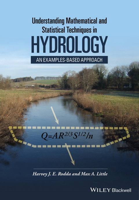
Understanding Mathematical and Statistical Techniques in Hydrology (eBook)

An Examples-based Approach

Harvey J. E. Rodda, Max A. Little (Autoren)

eBook Download: EPUB

2015
John Wiley & Sons (Verlag)
978-1-119-07660-5 (ISBN)

Infos

Pick up any hydrology textbook and it will not be long before you encounter pages listing sequences of equations representing complex mathematical concepts. Students and practitioners of hydrology will not find this very helpful, as their aim, generally, is to study and understand hydrology, and not to find themselves confronted with material that even students of mathematics would find challenging. Often, equations appear to be copied and pasted into hydrological texts in an attempt to give a more rigorous scientific basis to the narrative. However, they are commonly wrong, poorly explained, without context or background, and more likely to confuse and distance the reader than to enlighten and engage them in the topic.
Understanding Mathematical and Statistical Techniques in Hydrology provides full and detailed expositions of such equations and mathematical concepts, commonly used in hydrology. In contrast to other hydrological texts, instead of presenting abstract mathematical hydrology, the essential mathematics is explained with the help of real-world hydrological examples.

Dr Harvey J. E. Rodda graduated in Environmental Science from Lancaster University and completed his PhD in the Department of Geography, Exeter University in 1993 in the field of hydrological modelling. He is currently a director of Hydro-GIS Ltd, a consultancy company providing specialist services in hydrology and GIS mostly within the private sector. Since 2005 he has been a visiting lecturer at University College London, Department of Earth Sciences, teaching a hydrology module as part of the Geophysical Hazards MSc course.
Professor Max A. Little began his career writing software, signal processing algorithms and music for video games, then moved on by way of a degree in mathematics to the University of Oxford. After postdoc positions in Oxford investigating rainfall and biophysical time series data, he won a Wellcome Trust fellowship at MIT to follow up on his doctoral research work in behavioural and biomedical signal processing. He is currently an associate professor of mathematics at Aston University and a visiting professor at MIT's Media Lab.

Inhalt

Preface vii

How to use this book x

1 Fundamentals 1

1.1 Motivation for this book 1

1.2 Mathematical preliminaries 2

2 Statistical modelling 19

2.1 The Central European Floods, August 2002 19

2.2 Extreme value analysis 22

2.3 Simple methods of return period estimation 22

2.4 Return periods based on distribution fitting 25

2.5 Techniques for parameter estimation 30

2.6 Bayesian parameter estimation 30

2.7 Resampling methods: bootstrapping 31

3 Mathematics of hydrological processes 34

3.1 Introduction 34

3.2 Algebraic and difference equation methods 34

3.3 Methods involving exponentiation 36

3.4 Rearranging model equations 36

3.5 Equations with iterated summations and products 38

3.6 Methods involving differential equations 41

3.7 Methods involving integrals 43

4 Techniques based on data fitting 45

4.1 Experimental and observed data 45

4.2 Rating curves 46

4.3 Regression with two or more independent variables 49

4.4 Demonstration of decaying quantities 51

4.5 Analysis based on harmonic functions 52

5 Time series data 55

5.1 Introduction 55

5.2 Characteristics of time series data 55

5.3 Testing for time dependence 57

5.4 Testing for trends 58

5.5 Frequency analysis 59

5.6 Other analysis methods 60

5.7 Smoothing and filtering 60

5.8 Linear smoothing and filtering methods 61

5.9 Nonlinear filtering methods 64

5.10 Time series modelling 66

5.11 Hybrid time series/process-based models 67

5.12 Detecting non-stationarity 69

6 Measures of model performance, uncertainty and stochastic modelling 71

6.1 Introduction 71

6.2 Quantitative measures of performance 71

6.3 Comparing measures 73

6.4 The Nash-Sutcliffe method 75

6.5 Stochastic modelling 76

6.6 Monte Carlo simulations 77

6.7 Non-uniform Monte Carlo sampling 79

6.8 Uncertainty in hydrological modelling 81

6.9 Uncertainty in combined models 82

6.10 Assessing uncertainty given observed data: Bayesian methods 83

Glossary 86

Index 88

Textauszug

CHAPTER 1
Fundamentals

1.1 Motivation for this book

Hydrology is the study of water, and in the International Glossary of Hydrology (UNESCO/WMO 1992) it is defined as ‘Science that deals with the waters above and below the land surfaces of the Earth, their occurrence, circulation and distribution, both in space and time, their biological, chemical and physical properties, their reaction with their environment, including their relation to living beings’. The movement and transformation of water within these processes as described in the definition, as a fluid, will obey the physical rules of fluid mechanics. Fluid mechanics, being a quantitative topic, requires heavy use of mathematical concepts, and these concepts are therefore naturally found in hydrology. These quite basic physical principles can be used effectively to model and hence predict and understand the behaviour of water under many useful circumstances.

Nonetheless, despite the essentially predictable behaviour of water that justifies the use of mathematical principles, often, the flow of water in practice is subject to forces that are beyond our ability to measure with any precision: for example, water in the atmosphere is heated, cooled, mixed with numerous gasses, and transported across large distances under the action of turbulent winds. Eventually, water condenses out of the atmosphere in the form of precipitation but exactly when, where, and how much water falls to the ground under gravity is often extremely uncertain. This uncertainty usually makes it useless to apply the basic physical principles of fluid mechanics to the flow of water in these circumstances. For this reason, hydrologists often turn to statistics, which can be considered as the application of mathematics to uncertain phenomena.

Quantitative hydrology is, therefore, based on an interesting mix of the two great branches of applied mathematics: physical laws (mathematical physics) and probability (mathematical statistics).

Mathematics is, perhaps, the archetypal example of a composite subject. This means that more complex concepts are built from many simpler ones, and so, in order to properly understand the more complex topic, it is necessary to understand the simpler ones from which it is constructed. Not all subjects are like this: it is possible to gain a deep understanding of many aspects of plant biology without having to know anything about mammals, for instance. But mathematics is unforgiving: one cannot understand the true meaning of equations of fluid transport without knowing calculus. Unfortunately, for many reasons, the chance to learn the basic mathematical concepts is not afforded to every student or practitioner of hydrology, and many find themselves at a loss when presented with more complex mathematical concepts as a result.

This book is therefore, intended as a guide to students and practitioners of hydrology without a formal or substantive background in either mathematical physics, or mathematical statistics, who need to gain a more thorough grounding of these mathematical techniques in practical hydrological applications.

1.2 Mathematical preliminaries

This book refers extensively to many essential, but nonetheless quite simple, mathematical concepts; we introduce them here. It is assumed that readers will refer back to this section on reading the later material.

1.2.1 Numbers and operations

Usually when one thinks of ‘mathematics’, one thinks of numbers, along with operations such as adding, subtracting, multiplying (forming the product) and dividing them. Numbers and operations are intimately related: for example, with the simplest of numbers, the whole numbers, we can answer questions such as ‘what number, when added to 5, gives 10?’ Symbolically, we wish to find the x that satisfies the equation , the answer being . But some simple questions involving whole numbers cannot be answered using whole numbers, for instance, the problem ‘what number, when added to 10, gives 5?’, or , has no whole number answer. To solve such a problem, we need to include negative numbers and zero; mathematicians call these whole numbers that can be negative, zero, or positive, the integers (all the positive whole numbers are included in the integers). Still, when faced with whole number problems involving multiplication, integers may not suffice. For example, the problem ‘what number, when multiplied by 5, equals 1?’, or , has no integer solution. The answer is called a rational number and all the integers are included in the rationals. Finally, it turns out that there are yet more problems involving multiplication that cannot be solved using rationals; consider the problem ‘what number, when multiplied by itself, equals 2?’ The corresponding equation is solved by the square root of 2, , which is an example of a real number. The set of real numbers includes all the rationals and numbers such as (which can never be written out to full precision because it has an infinite number of decimal places). With the set of all real numbers, a very large set of problems involving numbers and operations that do actually have a solution can be answered.

It is surprising that even in apparently simple situations such as multiplication and addition with whole numbers, that there are equations that have no solution in the rationals, let alone the integers and whole numbers. Such equations baffled mathematicians until the 19th century when a logically consistent foundation for the real number system was devised. But real numbers do not even suffice for all whole number equations! Consider the equation ; because squaring any number is always positive, there does not seem to be any way to choose a number for x that, when squared, gives a negative number to cancel the 2 and satisfy the equation. Nevertheless, it turns that a consistent solution is possible using complex numbers; although abstract, these can be useful in physical problems.

These days, because of their practical utility, real numbers tend to be the lifeblood of quantitative sciences including hydrology. For instance, the average amount of rainfall occurring in one day in one location is often given as a real number in millimetres, to a couple of decimal places where such precision is appropriate. Therefore, most practical problems in hydrology involve solutions that are real numbers given to some limited accuracy appropriate to the problem.

1.2.2 Algebra: rearranging expressions and equations

An important step in the historical development of mathematics was the leap from dealing with specific numbers, to dealing with any number by using an abstract symbol to stand for that number (this conceptual leap is usually credited to the great Islamic mathematicians of the medieval period). This is the topic of algebra: the study of what happens to these symbols as they are manipulated as if they were numbers. Most quantitative problems in the physical sciences can be expressed and solved algebraically.

Algebra involves very simple rules. Although the rules themselves are elementary, the consequences of those rules can be extremely complex; in fact, much research still goes on today to understand the full, logical consequences of algebra. For this reason, one should not underestimate how difficult it can be to correctly derive the consequences of any particular application of algebra in practice, and it is very much worth the effort to become as familiar as possible with the basic rules.

Today, one usually writes something like x or y when one wants to refer to an abstract number; these are also called variables (as opposed to specific numbers, which are constants). Then the notation is an algebraic expression using these two variables and the constant 1.

Expressions on their own do not ‘do’ anything; to make expressions useful we need to connect them together into equations, for instance, the equation states that if the variables x and y are added to the constant 1, then the result must be equal to zero. Alternatively, by manipulating (rearranging) this equation, we can get the exactly equivalent statement , which is obtained by subtracting 1 from both sides. This is an example of a basic rule in algebra: in order to rearrange an equation, one has to apply the same operation to both sides of an equation, step by step. This rule ensures that before and after the manipulation, the equation still has the same mathematical meaning.

These algebraic operations come in pairs – subtraction is the inverse of addition and division is the inverse of multiplication. What this means, roughly, is that subtraction ‘undoes’ addition and division ‘undoes’ multiplication. So, actually, what one is doing when rearranging an equation, is applying a sequence of inverse operation to both sides of an equation.

Rearranging equations is fundamental to the way in which answers to mathematical questions are obtained, often by finding the actual number (value) of some variable. For the equation , we only know the value of x and y implicitly (through the relationship created between them by the equality). However, it is often difficult (if not impossible) to find the value of x from an implicit equation. In this case, the solution is easy of course: rearrange the equation to find x alone on one side of the equation, for instance, (note that it...

Produkt-Details

• Erscheint lt. Verlag: 2.11.2015
• Sprache: englisch
• Themenwelt: Mathematik / Informatik ► Mathematik ► Statistik
• Themenwelt: Naturwissenschaften ► Geowissenschaften ► Hydrologie / Ozeanografie
• Themenwelt: Technik
• Schlagworte: Data Analysis • earth science • earth sciences • Environmental Statistics & Environmetrics • Flooding • flood science • Geology • Geophysical Hazards • Geophysics • geoscience • Geowissenschaften • groundwater • Groundwater & Hydrogeology • Grundwasser • Grundwasser u. Hydrogeologie • harvey rodda • hydrogeology • Hydrological Sciences • Hydrology • hydromodeling • Limnology • max little • mechanistic modeling • Oceanography • River Science • statistical hydrology • statistical modeling • Statistics • Statistik • time series data • Time Series Modeling • Umweltstatistik • Umweltstatistik u. Environmetrics • water resources
• ISBN-10: 1-119-07660-9 / 1119076609
• ISBN-13: 978-1-119-07660-5 / 9781119076605