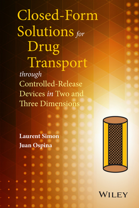
Closed-form Solutions for Drug Transport through Controlled-Release Devices in Two and Three Dimensions (eBook)

Laurent Simon, Juan Ospina (Autoren)

eBook Download: EPUB

2015
John Wiley & Sons (Verlag)
9781119055952 (ISBN)

Infos

Provides solutions for two- and three-dimensional linear models of controlled-release systems

• Real-world applications are taken from used to help illustrate the methods in Cartesian, cylindrical and spherical coordinate systems
• Covers the modeling of drug-delivery systems and provides mathematical tools to evaluate and build controlled-release devices
• Includes classical and analytical techniques to solve boundary-value problems involving two- and three-dimensional partial differential equations
• Provides detailed examples, case studies and step-by-step analytical solutions to relevant problems using popular computational software

Laurent Simon, PhD, is Associate Professor of Chemical Engineering and served as the Associate Director of the Pharmaceutical Engineering Program at New Jersey Institute of Technology. Dr. Simon is the author of Laboratory Online, a series of educational and interactive modules that help engineers build a strong understanding of drug delivery technologies and their underlying engineering principles. During his time at NJIT, Dr. Simon has received the Excellence in Teaching Award, Master Teacher Designation, Newark College of Engineering Saul K. Fenster Innovation in Engineering Education Award and a Distinguished Teaching Award from the American Society of Engineering Education (ASEE).
Juan Ospina is currently an Assistant Professor at EAFIT University in the Logic and Computation Group, Physics Engineering Program. He has published numerous articles on the topic of mathematical physics.

Textauszug

1
STEADY-STATE ANALYSIS OF A TWO-DIMENSIONAL MODEL FOR PERCUTANEOUS DRUG TRANSPORT

1.1 SEPARATION OF VARIABLES IN 2-D CARTESIAN COORDINATES

The Laplace's equation in two-dimensional Cartesian coordinates takes the form

(1.1)

which is solved to give

(1.2)

where and are arbitrary functions of and , respectively, and . This solution can be obtained in Maple using the command pdsolve. However, Eq. (1.2) is rarely used, in practice. Instead, the method of separation of variables is adopted. The goal of this technique is to reduce the original problem into a system of ordinary differential equations in one variable (Rice & Do, 1995).

A solution of Eq. (1.1) is . These two functions satisfy the equations

(1.3)

and

(1.4)

where represents an arbitrary constant. After solving Eqs. (1.3) and (1.4) for and , we obtain

(1.5)

The solution (1.5) is expressed as an additive separation of variables (Cherniavsky, 2010). Another method for solving Eq. (1.1) is the use of a multiplicative separation of variables such that . In this case, and satisfy the following ordinary differential equations:

(1.6)

and

(1.7)

After solving Eqs. (1.6) and (1.7), the solution is

(1.8)

Given that is an arbitrary constant, it is possible to apply the principle of superposition (Farlow, 1993) to get

(1.9)

The discrete form of Eq. (1.9) is

(1.10)

The types of boundary conditions determine the choice of Eq. (1.9) or (1.10). In cases where Eqs. (1.5) and (1.9) are both solutions, their sum is also a solution:

(1.11)

or

(1.12)

after using the discretized form of Eq. (1.9).

1.2 MODEL FOR DRUG TRANSPORT ACROSS THE SKIN

The steady-state drug transport across the skin is described by Laplace's equation (1.1). The drug is contained in a patch of length (Fig. 1.1). During treatment, the drug concentration in the reservoir remains unchanged (Simon & Ospina, 2013). Two segments perpendicular to the skin surface, and , are chosen in this application. There is no exchange of material with the environment except at the skin/capillary boundary. A first-order elimination kinetics is observed at the interface. After using the dimensionless variables and constants,

(1.13)

Figure 1.1 Diagram of the drug absorption model.

the boundary conditions are

(1.14)

(1.15)

(1.16)

(1.17)

where

(1.18)

and “Heaviside(y − a)” is the step function defined as

(1.19)

The coefficients and are the drug diffusivity and clearance at the skin/capillary boundary; and are the concentrations in the reservoir and in the skin, respectively. Also,

(1.20)

Note that Eq. (1.14) is equivalent to the following three conditions:

(1.21)

(1.22)

and

(1.23)

1.3 ANALYTICAL SOLUTION OF THE DIFFUSION MODEL IN 2-D CARTESIAN SYSTEMS

We look for a solution to Eq. (1.1) of the form (i.e., multiplicative separation of variables). Eq (1.8) is used in this case. Condition (1.15) leads to

(1.24)

Replacing Eq. (1.24) in Eq. (1.8) and applying condition (1.16) yield

(1.25)

leading to

(1.26)

Equation (1.8) becomes

(1.27)

Given that there is a solution for every value of , we write

(1.28)

Applying the principle of superposition for linear equations, we have

(1.29)

The use of condition (1.17) in Eq. (1.29) results in

(1.30)

Therefore, the concentration is

(1.31)

Finally, after applying Eq. (1.14) to Eq. (1.31), we have

(1.32)

The solution to the problem, defined by Eqs. (1.1), (1.14), (1.15), (1.16), (1.17), is given by Eqs. (1.31) and (1.32). Using Eq. (1.32), it is possible to develop successive approximations. For example, a zero-order solution can be obtained by setting with . In this case, Eq. (1.31) reduces to

(1.33)

The coefficient is calculated from Eq. (1.32) resulting in the following “zero-order” approximation of the concentration (Fig. 1.2):

(1.34)

Figure 1.2 Normalized drug concentration in the skin: , , , and .

1.4 SUMMARY

The method of separation of variables was applied to solve Laplace's equation in two dimensions. In this technique, the partial differential equation is reduced to ordinary differential equations in one variable. The principle of linear superposition was implemented to add the solutions of the subproblems and generate the solution of the initial PDE model. This procedure helps derive the spatial distribution of drug across the skin.

1.5 APPENDIX: MAPLE, MATHEMATICA, AND MAXIMA CODE LISTINGS

1.5.1 Maple Code: steadytwo.mws

________________________________________________________________ > restart:with(VectorCalculus):with(PDETools); > eq:=Laplacian(c(x,y),cartesian[x,y])=0; > eq1:=alpha(y)*c(0,y)+beta(y)*Eval(diff(c(x,y),x),x=0)=delta(y): > eq2:=Eval(diff(c(x,y),y),y=−L[d])=0: > eq3:=Eval(diff(c(x,y),y),y=L[u])=0: > eq4:=Eval(diff(c(x,y),x),x=1)+w*c(1,y)=0: > eq5:=pdsolve(eq,HINT=f(x)*g(y)): > eq6:=factor(build(eq5)): > eq7:=eval(diff(rhs(eq6),y),y=−L[d])=0: > > eq8:=isolate(eq7,_C4): > eq9:=factor(subs(eq8,eq6)): > eq10:=subs(_C3=1,eq9): > eq11:=factor(combine((eq10),sin)): > eq12:=eval(diff(rhs(eq11),y),y=L[u])=0: > eq13:=sin(_c[1]ˆ(1/2)*(L[u]+L[d]))=0: > > eq14:=_c[1]ˆ(1/2)*(L[u]+L[d])=n*Pi: > eq15:=isolate(eq14,_c[1]): > eq16:=simplify(subs(eq15,eq11),power,symbolic): > eq17:=subs(_C1=A[n],_C2=B[n],c=c[n],eq16): > eq18:=c(x,y)=Sum(rhs(eq17),n=0..infinity); > > eq22:=subs(c=c[n],eq4): > > eq23:=subs(x=1,eq17): > eq24:=factor(eval(subs(Eval=eval,subs(eq23,subs(eq17,eq22))))): > eq25:=simplify(simplify(factor(isolate(eq24,B[n])),power,symbolic),exp): > eq26:=collect(subs(eq25,eq17),A[n]): > eq26A:=subs(n=0,simplify(series(rhs(eq26),n=0,4))): > eq27:=c(x,y)=eq26A+Sum(rhs(eq26),n=1..infinity): > > eq19:=eq1: > > eq19A:=eval(subs(x=0,eq27)): > eq20:=factor(eval(subs(Eval=eval,subs(eq19A,subs(eq27,eq19))))): > ============= Zero‐order approximation====================== > eq28:=factor(eval(subs(Sum=sum,subs(A[n]=0,eq20)))): > eq29:=simplify(subs(y=z,Int(lhs(eq28),y=−L[d]..L[u])=Int(rhs(eq28),y=−L[d]..L[u]))): > eq30:=isolate(eq29,A[0]): > eq31:=eval(subs(Sum=sum,subs(A[n]=0,eq27))): > eq32:=subs(eq30,eq31): > ñas:=alpha(y)=Heaviside(y)‐Heaviside(y‐L[c]): > ñasA:=beta(y)=alpha(y)‐1: > ñasB:=delta(y)=alpha(y): > eq32A:=subs(y=z,ñas): > eq32B:=subs(y=z,ñasA): > eq32C:=subs(y=z,ñasB): > eq32D:=eval(subs(Int=int,subs(eq32A,subs(eq32C,eq32B,eq32)))) assuming L[c]>0 and L[d]>0 and L[u]>0 and L[u]>L[c]; > ______________________________________________________________________

1.5.2 wxMaxima Code: steadytwo.wxm

_____________________________________________________________________ (%i1) eq: diff(C(x,y),x,2)+diff(C(x,y),y,2)=0; (%i2)...

Produkt-Details

• Erscheint lt. Verlag: 13.7.2015
• Sprache: englisch
• Themenwelt: Medizin / Pharmazie ► Gesundheitsfachberufe
• Themenwelt: Medizin / Pharmazie ► Medizinische Fachgebiete ► Pharmakologie / Pharmakotherapie
• Themenwelt: Naturwissenschaften ► Chemie ► Technische Chemie
• Themenwelt: Technik ► Umwelttechnik / Biotechnologie
• Schlagworte: biomedical engineering • Biomedizintechnik • chemical engineering • Chemie • Chemische Verfahrenstechnik • Chemistry • closed-form solution • Controlled-release system • Drug Formulation & Delivery • Physiologic Modeling & Control Systems • Physiologische Modellierung, Steuersysteme • three-dimensional model • Two-Dimensional Model • Wirkstoffformulierung, Wirkstofftransport
• ISBN-13: 9781119055952 / 9781119055952