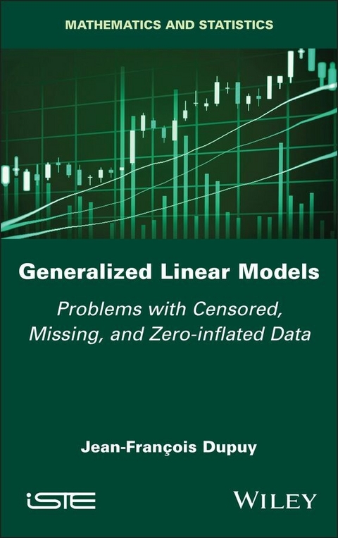
Generalized Linear Models (eBook)

Problems with Censored, Missing, and Zero-inflated Data

Jean-Francois Dupuy (Autor)

eBook Download: EPUB

2025
322 Seiten
Wiley-Iste (Verlag)
978-1-394-38844-8 (ISBN)

Infos

Since they were first formulated in 1972, generalized linear models have enjoyed a veritable boom, with numerous applications in insurance, economics and biostatistics. Today, they are still the subject of a great deal of research.

This book provides an overview of the theory of generalized linear models. Particular attention is paid to the problems of censoring, missing data and excess zeros. Didactic and accessible, Generalized Linear Models is illustrated with exercises and numerous R codes.

With all the necessary prerequisites introduced in a step-by-step fashion, this book is aimed at students (at master's or engineering school level), as well as teachers and practitioners of mathematics and statistical modeling.

Jean-François Dupuy is Professor of Applied Mathematics at the University of Rennes and is a member of the Institut de recherche mathématique de Rennes, France. His research focuses on statistical modeling, generalized linear models and duration models.

Textauszug

1
Exponential Families

Exponential families play a central role in the construction of generalized linear models (Chapter 2). This first chapter is dedicated to them. We will limit ourselves to the results that are strictly necessary to understand the rest of the book. The interested reader will find a more detailed exposition in Sundberg (2019).

1.1. Definition

Recall that a statistical model is a pair , where is a set (called the space of observations) and is a family of probability distributions on . A statistical model is said to be parametric if the family can be described by a parameter θ that lives in a finite-dimensional vector space, typically ℝp where p ∈ ℕ* (or in a subspace Θ of this vector space). In the contrary case, a model is said to be non-parametric. A parametric model will be denoted in the following way:

or, more simply, if we omit :

The space Θ is called the parameter space. For example, the family of normal distributions with mean m and variance σ2 constitutes a parametric model for a real observation. The family of Poisson distributions with parameter µ is a parametric model for an integer-valued observation (called count or enumeration).

A parametric statistical model (where Θ ⊆ ℝ) is said to be an exponential model if the distribution Pθ,ϕ admits a density (with respect to a suitable dominant measure µ: the Lebesgue measure on ℝ or a subinterval of ℝ, or the counting measure on a countable set) of the form:

[1.1]

where a(·) and b(·, ·) are functions which determine which particular model is being considered (Poisson model, Gaussian model, etc.), as we will see in section 1.3.

The parameter θ is said to be the canonical parameter of the model (we sometimes also call it the natural parameter, but this last term is not very appropriate since the canonical parameter does not strongly correspond to the most natural parameterization of the model; see section 1.3).

The parameter ϕ, called the dispersion parameter, is often considered to be a nuisance parameter, with θ being the parameter of interest within the model. The family of densities is called an exponential family.

REMARK.– In the literature, we will encounter definitions of the exponential model, which uses slightly different forms of the density [1.1]. For example, in the denominator of [1.1], ϕ is sometimes replaced by a function c(ϕ), which itself is often expressed in the form c(ϕ) = ϕ/ω, where ω is a known weight. In order to keep the notation simple, in this book, we will adopt the parameterization in [1.1], since it encompasses the most common examples of exponential families (an example in which a weight ω occurs is described in Chapter 2).

If ϕ is known (e.g. when ϕ = 1 in the binomial and Poisson distributions), we can set:

so that [1.1] becomes:

[1.2]

which is an expression for the density that is commonly used to define the exponential model. The quantity C(θ) here plays the role of a normalization constant, making the function f(y; θ) into a probability density (we have ).

1.2. Mean, variance, and variance function

Let Y be a random variable with density [1.1]. Additionally, set and (we will assume that a is infinitely differentiable; see Sundberg (2019)). We will now show the following result:

PROPOSITION 1.1.– In the model [1.1], we have:

REMARK.– Since the function is continuous and strictly increasing on Θ (since ), it therefore admits a continuous inverse, .

PROOF OF PROPOSITION 1.1.– Let us set , and assume that we can interchange the integral and differential operators. To simplify the notation below, we will write in the place of and dy in the place of dµ(y).

Using this notation:

and:

since . Now, we differentiate [1.1] twice with respect to θ to obtain successively:

and:

Now, integrate these two expressions with respect to y. We obtain:

From the first equation, we immediately deduce that and, by observing that , we easily deduce from the second equation that var(Y ) = ϕä(θ).

In the following, we will set , so that with this notation:

where . The function v(µ) is called the variance function. In the model [1.1], it describes the way in which the variance of Y varies as a function of its mean (this is said to be the mean-variance relation).

In the Gaussian model, we will see in section 1.3 that v(µ) = 1. Therefore, v(µ) does not depend on µ: the variance and the mean vary independently from one another. For the Poisson distribution, v(µ) = µ: the variance varies like the expected value. For the gamma distribution, v(µ) = µ2: the variance varies like the square of the expected value (the standard deviation varies like the expected value).

1.3. Examples of exponential families

Exponential families include many of the classical probability distributions. We will describe some examples below, though there exists a great deal more examples (Sundberg 2019).

EXAMPLE 1.1 (BINOMIAL DISTRIBUTION).– Let k ∈ ℕ* be fixed. The family of binomial distributions with parameter π is an exponential family. Indeed, with respect to the counting measure on {0, 1, …, k}, for the distribution, we have:

which can be identified with [1.1], if we set and .

We see that:

and:

Denoting , then the variance function is equal to: v(µ) = µ(k – µ)/k.

REMARK.– The particular case when k = 1 corresponds to the Bernoulli distribution. We will denote it by .

EXAMPLE 1.2 (POISSON DISTRIBUTION).– The family of Poisson distributions with parameter µ is an exponential family. The density on ℕ for the distribution is written as:

We identify it with [1.1] by setting θ = ln µ, ϕ = 1, a(θ) = µ = eθ and b(y, θ) = –ln y!. We see that:

We recover the equality property (called equidispersion) of the mean and variance from the Poisson distribution. Finally, the variance function v(µ) is simply equal to v(µ) = µ.

EXAMPLE 1.3 (NEGATIVE BINOMIAL DISTRIBUTION).– Let us consider a series of independent events in which a “success” occurs with constant probability π (so that “failure” occurs with complementary probability 1 – π). We repeat the events until a given number of k successes (with k ∈ {1, 2, …}) have occurred. The negative binomial distribution is the probability distribution of the random variable Y that counts the number of failures, which have occurred before obtaining k successes.

Its probability density is written as:

REMARK.– The particular case when k = 1 corresponds to the geometric distribution.

For each integer n, recall that Γ(n + 1) = n!, and set κ = 1/k and . We can then rewrite f as follows:

[1.3]

and then again, after some simple calculations:

We identify f with [1.1] by setting and . The negative binomial distributions therefore form an exponential family. We see that:

and:

The variance function is equal to:

The mean-variance relation is thus quadratic, from which comes the name “NB2 distribution” which is sometimes given to this distribution (the “2” refers to the power of µ in the variance function) (Cameron and Trivedi 1998; Hilbe 2011).

There exists another parameterization of the negative binomial distribution, in which the variance is a linear function of the mean. The corresponding distribution is hence called the “NB1 distribution”.

The NB2 distribution can be obtained as a Poisson–gamma mixture (we show this in the technical appendix to this chapter; see section 1.5). This interpretation, along with the fact that , make the negative binomial distribution a very useful model for overdispersed count data.

EXAMPLE 1.4 (NORMAL DISTRIBUTION).– The family of normal distributions with mean µ and variance σ2 form an exponential family. The distribution has the following density on ℝ:

which can be identified with [1.1] if we set and . We see that:

The variance function is equal to v(µ) = 1.

EXAMPLE 1.5 (GAMMA DISTRIBUTION).– The family of gamma distributions form...

Produkt-Details

• Erscheint lt. Verlag: 17.6.2025
• Reihe/Serie: ISTE Invoiced
• Sprache: englisch
• Themenwelt: Mathematik / Informatik ► Mathematik ► Statistik
• Themenwelt: Mathematik / Informatik ► Mathematik ► Wahrscheinlichkeit / Kombinatorik
• Schlagworte: Biostatistics • Data Analysis • Economics • generalized linear modeling • zero-inflated data
• ISBN-10: 1-394-38844-6 / 1394388446
• ISBN-13: 978-1-394-38844-8 / 9781394388448