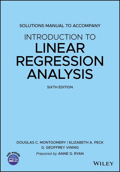
Introduction to Linear Regression Analysis, 6e Solutions Manual (eBook)

Douglas C. Montgomery, Elizabeth A. Peck, G. Geoffrey Vining (Autoren)

eBook Download: EPUB

2022 | 6. Auflage
John Wiley & Sons (Verlag)
978-1-119-57876-5 (ISBN)

Infos

A comprehensive and current introduction to the fundamentals of regression analysis Introduction to Linear Regression Analysis, 6th Edition is the most comprehensive, fulsome, and current examination of the foundations of linear regression analysis. Fully updated in this new sixth edition, the distinguished authors have included new material on generalized regression techniques and new examples to help the reader understand retain the concepts taught in the book. The new edition focuses on four key areas of improvement over the fifth edition: New exercises and data sets New material on generalized regression techniques The inclusion of JMP software in key areas Carefully condensing the text where possible Introduction to Linear Regression Analysis skillfully blends theory and application in both the conventional and less common uses of regression analysis in today's cutting-edge scientific research. The text equips readers to understand the basic principles needed to apply regression model-building techniques in various fields of study, including engineering, management, and the health sciences.

Autor

DOUGLAS C. MONTGOMERY, PHD, is Regents Professor of Industrial Engineering and Statistics at Arizona State University. Dr. Montgomery is the co-author of several Wiley books including Introduction to Linear Regression Analysis, 5th Edition. ELIZABETH A. PECK, PHD, is Logistics Modeling Specialist at the Coca-Cola Company in Atlanta, Georgia. G. GEOFFREY VINING, PHD, is Professor in the Department of Statistics at Virginia Polytechnic and State University. Dr. Peck is co-author of Introduction to Linear Regression Analysis, 5th Edition.

Inhalt

Preface vii

2 Simple Linear Regression 1

3 Multiple Linear Regression 13

4 Model Adequacy Checking 29

5 Transformations and Weighting to Correct Model Inadequacies 59

6 Diagnostics for Leverage and Influence 74

7 Polynomial Regression Models 79

8 Indicator Variables 86

9 Multicollinearity 95

10 Variable Selection and Model Building 100

11 Validation of Regression Models 105

12 Introduction to Nonlinear Regression 108

13 Generalized Linear Models 113

14 Regression Analysis of Time Series Data 121

15 Other Topics in the Use of Regression Analysis 125

Textauszug

Chapter 3
Multiple Linear Regression

1. 3.1
   1. .
   2. Regression is significant.

      Source	d.f.	SS	MS	F	p-value

      Regression

      3

      257.094

      85.698

      29.44

      0.000

      Error

      24

      69.87

      2.911

      Total

      27

      326.964

   3. All three are significant.

      Coefficient	test statistic	p-value

      β2

      5.18

      0.000

      β7

      2.20

      0.038

      β8

      −3.77

      0.001

   4. R2 = 78.6% and
   5. F0 = (257.094 − 243.03)/2.911 = 4.84 which is significant at α = 0.05. The test statistic here is the square of the t-statistic in part c.

1. 3.2 Correlation coefficient between yi and is .887. So (.887)2 = .786 which is R2.
2. 3.3
   1. A 95% confidence interval on the slope parameter β7 is
   2. A 95% confidence interval on the mean number of games won by a team when x2 = 2300, x7 = 56.0 and x8 = 2100 is
3. 3.4
   1. with F = 15.13 and p = 0.000 which is significant.
   2. R2 = 54.8% and which are much lower.
   3. For β7, a 95% confidence interval is 0.484 ± 2.064(.1192) = (−.198, .294) and for the mean number of games won by a team when x7 = 56.0 and x8 = 2100, a 95% confidence interval is 6.926 ± 2.064(.533) = (5.829, 8.024). Both lengths are greater than when x2 was included in the model.
   4. It can affect many things including the estimates and standard errors of the coefficients and the value of R2.
4. 3.5
   1. Regression is significant.

      Source	d.f.	SS	MS	F	p-value

      Regression

      2

      972.9

      486.45

      53.31

      0.000

      Error

      29

      264.65

      9.13

      Total

      31

      1237.54

   2. R2 = 78.6% and . For the simple linear regression with x1, R2 = 77.2%.
   3. A 95% confidence interval for the slope parameter β1 is −.053 ± 2.045(.006145) = (−.0656, −.0405).
   4. x1 is significant while x6 is not.

      Coefficient	test statistic	p-value

      β1

      −8.66

      0.000

      β6

      1.43

      0.163

   5. A 95% confidence interval on the mean gasoline mileage when x1 = 275 in3 and x6 = 2 is 20.187 ± 2.045(.643) = (18.872, 21.503).
   6. A 95% prediction interval for a new observation on gasoline mileage when x1 = 275 in3 and x6 = 2 is 20.187 ± 2.045(3.089) = (13.887, 26.488)
5. 3.6 The lengths from problem 2.4 are 2.223 and 12.716, respectively. For problem 3.5, they are 2.631 and 12.634. The lengths are pretty much the same which indicates that adding x6 does not help much.
6. 3.7
   1. F = 9.04 with p = 0.000 which is significant.
   2. None of the t-tests are significant. There is a multicollinearity problem.
   3. which indicates their is no contribution of lot size and living space given that all the other regressors are in the model.
   4. Yes, there is a multicollinearity problem.
7. 3.8
   1. F = 27.95 with p = 0.000 which is significant. R2 = 70.0% and .
   2. Both are significant.

      Coefficient	test statistic	p-value

      β6

      6.74

      0.000

      β7

      2.25

      0.034

   3. For β6, a 95% confidence interval is .0185 ± 2.064(.0027) = (.013, .024) and for β7, a 95% confidence interval is 2.185 ± 2.064(.9727) = (.177, 4.193).
   4. t = 6.62 with p = 0.000 which is significant. R2 = 63.6% and . These are basically the same as in part b.
   5. A 95% confidence interval on the slope parameter β6 is .019 ± 2.064(.0029) = (.013, .025). The length of this confidence interval is almost exactly the same as the one from the model including x7.
   6. As always, MSRes is lower when x6 and x7 are in the model.
8. 3.9
   1. F = 24.66 with p = 0.000 which is significant.
   2. R2 = 66.4% and
   3. x1 is significant while x4 is not.

      Coefficient	test statistic	p-value

      β1

      −5.12

      0.000

      β7

      −.02

      0.986

   4. It doesn't appear to be.
9. 3.10
   1. F = 16.51 with p = 0.000 which is significant.
   2. x4 and x5 appear to contribute to the model.

      Coefficient	test statistic	p-value

      β1

      1.35

      0.187

      β2

      1.77

      0.086

      β3

      0.82

      0.418

      β4

      3.84

      0.001

      β5

      −2.52

      0.017

   3. For the model in part a, R2 = 72.1% and . For the model with only aroma and flavor, R2 = 65.9% and . These are basically the same.
   4. For the model in part a, the confidence interval is 1.1683 ± 2.0369(.3045) = (.548, 1.789). For the model with only aroma and flavor, the confidence interval is 1.1702 ± 2.0301(.2905) = (.581, 1.759). These two intervals are almost the same.
10. 3.11
    1. F = 29.86 with p = 0.000 which is significant.
    2. x2 and x5 appear to contribute to the model.

       Coefficient	test statistic	p-value

       β1

       1.86

       0.093

       β2

       4.90

       0.001

       β3

       0.31

       0.763

       β4

       −0.00

       1.00

       β5

       −11.03

       0.000

    3. For the model in part a, R2 = 93.7% and . For the model with only temperature and particle size, R2 = 91.5% and . These are basically the same.
    4. For the model in part a, a 95% confidence interval is .282 ± 2.228(.05761) = (.154, .410). For the model with only aroma and flavor, a 95% confidence interval is .282 ± 2.16(.05883) = (.155, .409). These two intervals are almost the same.
11. 3.12
    1. F = 87.6 with p = 0.000 which is significant.
    2. Both contribute to the model.

       Coefficient	test statistic	p-value

       β1

       8.82

       0.000

       β2

       10.91

       0.000

    3. For the model in part a, R2 = 84.2% and . For the model with only time, R2...

Produkt-Details

• Erscheint lt. Verlag: 12.7.2022
• Mitarbeit: Sonstige Mitarbeit: Anne G. Ryan
• Sprache: englisch
• Themenwelt: Mathematik / Informatik ► Mathematik ► Statistik
• Themenwelt: Mathematik / Informatik ► Mathematik ► Wahrscheinlichkeit / Kombinatorik
• Schlagworte: Applications • basic inference problems • conventional linear regression • intro to linear regression analysis • Lineare Regression • Polynomial Regression • Regression Analysis • regression modeling introduction • Regressionsanalyse • resolve problems model inadequacy • Statistics • Statistik • uncommon linear regression
• ISBN-10: 1-119-57876-0 / 1119578760
• ISBN-13: 978-1-119-57876-5 / 9781119578765