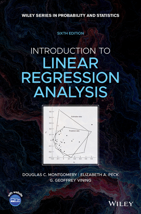
Introduction to Linear Regression Analysis (eBook)

Douglas C. Montgomery, Elizabeth A. Peck, G. Geoffrey Vining (Autoren)

eBook Download: EPUB

2021 | 6. Auflage
John Wiley & Sons (Verlag)
978-1-119-57875-8 (ISBN)

Infos

INTRODUCTION TO LINEAR REGRESSION ANALYSIS

A comprehensive and current introduction to the fundamentals of regression analysis

Introduction to Linear Regression Analysis, 6th Edition is the most comprehensive, fulsome, and current examination of the foundations of linear regression analysis. Fully updated in this new sixth edition, the distinguished authors have included new material on generalized regression techniques and new examples to help the reader understand retain the concepts taught in the book.

The new edition focuses on four key areas of improvement over the fifth edition:

New exercises and data sets

New material on generalized regression techniques

The inclusion of JMP software in key areas

Carefully condensing the text where possible

Introduction to Linear Regression Analysis skillfully blends theory and application in both the conventional and less common uses of regression analysis in today's cutting-edge scientific research. The text equips readers to understand the basic principles needed to apply regression model-building techniques in various fields of study, including engineering, management, and the health sciences.

DOUGLAS C. MONTGOMERY, PHD, is Regents Professor of Industrial Engineering and Statistics at Arizona State University. Dr. Montgomery is the co-author of several Wiley books including Introduction to Linear Regression Analysis, 5th Edition.

ELIZABETH A. PECK, PHD, is Logistics Modeling Specialist at the Coca-Cola Company in Atlanta, Georgia.

G. GEOFFREY VINING, PHD, is Professor in the Department of Statistics at Virginia Polytechnic and State University. Dr. Peck is co-author of Introduction to Linear Regression Analysis, 5th Edition.

Textauszug

CHAPTER 1
INTRODUCTION

1.1 REGRESSION AND MODEL BUILDING

Regression analysis is a statistical technique for investigating and modeling the relationship between variables. Applications of regression are numerous and occur in almost every field, including engineering, the physical and chemical sciences, economics, management, life and biological sciences, and the social sciences. Regression analysis is used extensively in data mining and is a basic tool of data science and analytics. Because of its wide applicability to a range of problems, regression analysis may be the most widely used statistical technique.

As an example of a problem in which regression analysis may be helpful, suppose that an industrial engineer employed by a soft drink beverage bottler is analyzing the product delivery and service operations for vending machines. He suspects that the time required by a route deliveryman to load and service a machine is related to the number of cases of product delivered. The engineer visits 25 randomly chosen retail outlets having vending machines, and the in-outlet delivery time (in minutes) and the volume of product delivered (in cases) are observed for each. The 25 observations are plotted in Figure 1.1a. This graph is called a scatter diagram. This display clearly suggests a relationship between delivery time and delivery volume; in fact, the impression is that the data points generally, but not exactly, fall along a straight line. Figure 1.1b illustrates this straight-line relationship.

If we let y represent delivery time and x represent delivery volume, then the equation of a straight line relating these two variables is

(1.1)

Figure 1.1 (a) Scatter diagram for delivery volume. (b) Straight-line relationship between delivery time and delivery volume.

where β0 is the intercept and β1 is the slope. Now the data points do not fall exactly on a straight line, so Eq. (1.1) should be modified to account for this. Let the difference between the observed value of y and the straight line (β0 + β1x) be an error ε. It is convenient to think of ε as a statistical error; that is, it is a random variable that accounts for the failure of the model to fit the data exactly. The error may be made up of the effects of other variables on delivery time, measurement errors, and so forth. Thus, a more plausible model for the delivery time data is

(1.2)

Equation (1.2) is called a linear regression model. Customarily x is called the independent variable and y is called the dependent variable. However, this often causes confusion with the concept of statistical independence, so we refer to x as the predictor or regressor variable and y as the response variable. Because Eq. (1.2) involves only one regressor variable, it is called a simple linear regression model.

To gain some additional insight into the linear regression model, suppose that we can fix the value of the regressor variable x and observe the corresponding value of the response y. Now if x is fixed, the random component ε on the right-hand side of Eq. (1.2) determines the properties of y. Suppose that the mean and variance of ε are 0 and σ2, respectively. Then the mean response at any value of the regressor variable is

Notice that this is the same relationship that we initially wrote down following inspection of the scatter diagram in Figure 1.1a. The variance of y given any value of x is

Thus, the true regression model μy|x = β0 + β1x is a line of mean values, that is, the height of the regression line at any value of x is just the expected value of y for that x. The slope, β1 can be interpreted as the change in the mean of y for a unit change in x. Furthermore, the variability of y at a particular value of x is determined by the variance of the error component of the model, σ2. This implies that there is a distribution of y values at each x and that the variance of this distribution is the same at each x.

Figure 1.2 How observations are generated in linear regression.

Figure 1.3 Linear regression approximation of a complex relationship.

For example, suppose that the true regression model relating delivery time to delivery volume is μy|x = 3.5 + 2x, and suppose that the variance is σ2 = 2. Figure 1.2 illustrates this situation. Notice that we have used a normal distribution to describe the random variation in ε. Since y is the sum of a constant β0 + β1x (the mean) and a normally distributed random variable, y is a normally distributed random variable. For example, if x = 10 cases, then delivery time y has a normal distribution with mean 3.5 + 2(10) = 23.5 minutes and variance 2. The variance σ2 determines the amount of variability or noise in the observations y on delivery time. When σ2 is small, the observed values of delivery time will fall close to the line, and when σ2 is large, the observed values of delivery time may deviate considerably from the line.

In almost all applications of regression, the regression equation is only an approximation to the true functional relationship between the variables of interest. These functional relationships are often based on physical, chemical, or other engineering or scientific theory, that is, knowledge of the underlying mechanism. Consequently, these types of models are often called mechanistic models. For example, the familiar physics equation momentum = mass × velocity is a mechanistic model.

Regression models, on the other hand, are thought of as empirical models. Figure 1.3 illustrates a situation where the true relationship between y and x is relatively complex, yet it may be approximated quite well by a linear regression equation. Sometimes the underlying mechanism is more complex, resulting in the need for a more complex approximating function, as in Figure 1.4, where a “piecewise linear” regression function is used to approximate the true relationship between y and x.

Generally regression equations are valid only over the region of the regressor variables contained in the observed data. For example, consider Figure 1.5. Suppose that data on y and x were collected in the interval x1 ≤ x ≤ x2. Over this interval the linear regression equation shown in Figure 1.5 is a good approximation of the true relationship. However, suppose this equation were used to predict values of y for values of the regressor variable in the region x2 ≤ x ≤ x3. Clearly the linear regression model is not going to perform well over this range of x because of model error or equation error.

Figure 1.4 Piecewise linear approximation of a complex relationship.

Figure 1.5 The danger of extrapolation in regression.

In general, the response variable y may be related to k regressors, x1, x2, …, xk, so that

(1.3)

This is called a multiple linear regression model because more than one regressor is involved. The adjective linear is employed to indicate that the model is linear in the parameters β0, β1, …, βk, not because y is a linear function of the x’s. We shall see subsequently that many models in which y is related to the x’s in a nonlinear fashion can still be treated as linear regression models as long as the equation is linear in the β’s.

An important objective of regression analysis is to estimate the unknown parameters in the regression model. This process is also called fitting the model to the data. We study several parameter estimation techniques in this book. One of these techmques is the method of least squares (introduced in Chapter 2). For example, the least-squares fit to the delivery time data is

where is the fitted or estimated value of delivery time corresponding to a delivery volume of x cases. This fitted equation is plotted in Figure 1.1b.

The next phase of a regression analysis is called model adequacy checking, in which the appropriateness of the model is studied and the quality of the fit ascertained. Through such analyses the usefulness of the regression model may be determined. The outcome of adequacy checking may indicate either that the model is reasonable or that the original fit must be modified. Thus, regression analysis is an iterative procedure, in which data lead to a model and a fit of the model to the data is produced. The quality of the fit is then investigated, leading either to modification of the model or the fit or to adoption of the model. This process is illustrated...

Produkt-Details

• Erscheint lt. Verlag: 24.2.2021
• Reihe/Serie: Wiley Series in Probability and Statistics
• Reihe/Serie: Wiley Series in Probability and Statistics
• Reihe/Serie: Wiley Series in Probability and Statistics
• Sprache: englisch
• Themenwelt: Mathematik / Informatik ► Mathematik ► Statistik
• Themenwelt: Mathematik / Informatik ► Mathematik ► Wahrscheinlichkeit / Kombinatorik
• Schlagworte: Angew. Wahrscheinlichkeitsrechn. u. Statistik / Modelle • Applied Probability & Statistics - Models • Data Analysis • Datenanalyse • Regression Analysis • Regressionsanalyse • Statistics • Statistik
• ISBN-10: 1-119-57875-2 / 1119578752
• ISBN-13: 978-1-119-57875-8 / 9781119578758