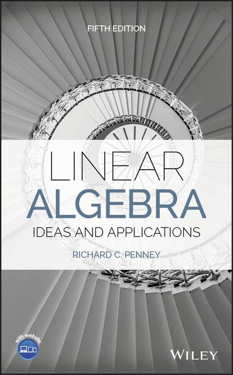
Linear Algebra (eBook)

Ideas and Applications

Richard C. Penney (Autor)

eBook Download: EPUB

2020 | 5. Auflage
John Wiley & Sons (Verlag)
978-1-119-65695-1 (ISBN)

Infos

Praise for the Third Edition

'This volume is ground-breaking in terms of mathematical texts in that it does not teach from a detached perspective, but instead, looks to show students that competent mathematicians bring an intuitive understanding to the subject rather than just a master of  applications.'

                  - Electric Review

Learn foundational and advanced topics in linear algebra with this concise and approachable resource

A comprehensive introduction, Linear Algebra: Ideas and Applications, Fifth Edition provides a discussion of the theory and applications of linear algebra that blends abstract and computational concepts. With a focus on the development of mathematical intuition, the book emphasizes the need to understand both the applications of a particular technique and the mathematical ideas underlying the technique. 

The book introduces each new concept in the context of explicit numerical examples, which allows the abstract concepts to grow organically out of the necessity to solve specific problems. The intuitive discussions are consistently followed by rigorous statements of results and proofs. Linear Algebra: Ideas and Applications, Fifth Edition also features:

• A new application section on section on Google's Page Rank Algorithm.
• A new application section on pricing long term health insurance at a Continuing Care Retirement Community (CCRC).
• Many other illuminating applications of linear algebra with self-study questions for additional study.
• End-of-chapter summaries and sections with true-false questions to aid readers with further comprehension of the presented material
• Numerous computer exercises throughout using MATLAB® code

Linear Algebra: Ideas and Applications, Fifth Edition is an excellent undergraduate-level textbook for one or two semester undergraduate courses in mathematics, science, computer science, and engineering.  With an emphasis on intuition development, the book is also an ideal self-study reference.

RICHARD C. PENNEY, PHD is Emeritus Professor in the Department of Mathematics and former Director of the Mathematics/Statistics Actuarial Science Program at Purdue University. He has authored numerous journal articles, received several major teaching awards, and is an active researcher. He received his graduate education at MIT.

Textauszug

CHAPTER 1
SYSTEMS OF LINEAR EQUATIONS

1.1 THE VECTOR SPACE OF m × n MATRICES

It is difficult to go through life without seeing matrices. For example, the 2019 annual report of Acme Squidget might contain the Table 1.1, which shows how much profit (in millions of dollars) each branch made from the sale of each of the company's three varieties of squidgets in 2019.

If we were to enter this data into a computer, we might enter it as a rectangular array without labels. Such an array is called a matrix. The Acme profits for 2019 would be described by the following matrix. This matrix is a matrix (read “five by four”) in that it has five rows and four columns. We would also say that its “size” is . In general, a matrix has size if it has rows and columns.

Definition 1.1  The set of all matrices is denoted .

TABLE 1.1 Profits: 2019

	Red	Blue	Green	Total

Kokomo

11.4

5.7

6.3

23.4

Philly

9.1

6.7

5.5

21.3

Oakland

14.3

6.2

5.0

25.5

Atlanta

10.0

7.1

5.7

22.8

Total

44.8

25.7

22.5

93.0

Each row of an matrix may be thought of as a matrix. The rows are numbered from top to bottom. Thus, the second row of the Acme profit matrix is the matrix

This matrix would be called the “profit vector” for the Philly branch. (In general, any matrix with only one row is called a row vector. For the sake of legibility, we usually separate the entries in row vectors by commas, as above.)

Similarly, a matrix with only one column is called a column vector. The columns are numbered from left to right. Thus, the third column of the Acme profit matrix is the column vector

This matrix is the “green squidget profit vector.”

If is a sequence of column vectors, then the matrix that has the as columns is denoted

Similarly, if is a sequence of row vectors, then the matrix that has the as rows is denoted

In general, if a matrix is denoted by an uppercase letter, such as , then the entry in the th row and th column may be denoted by either or , using the corresponding lowercase letter. We shall refer to as the “ entry of .” For example, for the matrix above, the entry is . Note that the row number comes first. Thus, the most general matrix is

We will also occasionally write “,” meaning that “ is the matrix whose entry is .”

At times, we want to take data from two tables, manipulate it in some manner, and display it in a third table. For example, suppose that we want to study the performance of each division of Acme Squidget over the two‐year period 2018–2019. We go back to the 2018 annual report, finding the 2018 profit matrix to be

If we want the totals for the two‐year period, we simply add the entries of this matrix to the corresponding entries from the 2018 profit matrix. Thus, for example, over the two‐year period, the Kokomo division made million dollars from selling blue squidgets. Totaling each pair of entries, we find the two‐year profit matrix to be

In matrix notation, we indicate that was obtained by summing corresponding entries of and by writing

In general, if and are matrices, then is the matrix defined by the formula

For example

Addition of matrices of different sizes is not defined.

What if, instead of totals for each division and each product, we wanted two‐year averages? We would simply multiply each entry of by . The notation for this is “.” Specifically,

In general, if is a number and is an matrix, we define

(1.1)

Hence,

There is also a notion of subtraction of matrices. In general, if and are matrices, then we define to be the matrix defined by the formula

Thus,

In linear algebra, the terms scalar and “number” mean essentially the same thing. Thus, multiplying a matrix by a real number is often called scalar multiplication.

The Space

We may think of a column vector as representing the point in the plane with coordinates . as in Figure 1.1. We may also think of as representing the vector from the point to —that is, as an arrow drawn from to . We will usually denote the set of matrices by when thought of as points in two‐dimensional space.

Like matrices, we can add pairs of vectors and multiply vectors by scalars. Specifically, if and are vectors with the same initial point, then is the diagonal of the parallelogram with sides and beginning at the same initial point (Figure 1.2b). For a positive scalar , is the vector with the same direction as that of , but with magnitude expanded (or contracted) by a factor of .

FIGURE 1.1 Coordinates in .

FIGURE 1.2 Vector Algebra.

Figure 1.2a shows that when two elements of are added, the corresponding vectors add as well. Similarly, multiplication of an element of by a scalar corresponds to multiplication of the corresponding vector by the same scalar. If , the direction of the vector is reversed and the vector is then expanded or contracted by a factor of (Figure 1.2b).

Example 1.1

Compute the sum of the vectors represented by and and draw a diagram illustrating your computation.

Solution.  The sum is computed as follows:

The vectors (along with their sum) are plotted in Figure 1.3.

FIGURE 1.3 Example 1.1.

FIGURE 1.4 Coordinates in .

Similarly, we may think of the matrix

as representing either the point in three‐dimensional space or the vector from to as in Figure 1.4. Matrix addition and scalar multiplication are describable as vector addition just as in two dimensions. We will usually denote the set of matrices by when thought of as points in three‐dimensional space.

What about matrices? Even though we cannot visualize dimensions, we still envision matrices as somehow representing points in dimensional space. The set of matrices will be denoted as when thought of in this way.

Definition 1.2  is the set of all matrices.

Linear Combinations and Linear Dependence

We can use our Acme Squidget profit matrices to demonstrate one of the most important concepts in linear algebra. Consider the last column of the 2019 profit matrix. Since this column represents the total profit for each branch, it is just the sum of the other columns in the profit matrix:

(1.2)

This last column does not tell us anything we did not already know in that we could have computed the sums ourselves. Thus, while it is useful to have the data explicitly displayed, it is not essential. We say that this data is “dependent on” the data in the other columns. Similarly, the last row of the profit matrix is dependent on the other rows in that it is just their sum.

For another example of dependence, consider the two profit matrices and and their average

(1.3)

The matrix depends on and —once we know and , we can compute .

These examples exhibit an especially simple form of dependence. In each case, the matrix we chose to consider as dependent was produced by multiplying the other matrices by scalars and adding. This leads to the following concept.

Definition 1.3  Let , be a set of elements of . An element of is linearly dependent on if there are scalars such that

(1.4)

We also say that “ is a linear combination of the .”

Remark.  In set theory, an object that belongs to a certain set is called an element of that set. The student must be careful not to confuse the terms “element” and “entry.” The matrix below is one element of the set of matrices. Every element of the set of matrices has four entries.

The expression “” means that is an element of the set .

One particular element of is linearly dependent on every other element of . This is the matrix, which has all its entries equal to 0. We denote this matrix by . It is referred to as “the zero element of .” Thus, the zero...

Produkt-Details

• Erscheint lt. Verlag: 8.12.2020
• Sprache: englisch
• Themenwelt: Mathematik / Informatik ► Mathematik ► Algebra
• Schlagworte: Algebra • Analytics • Angewandte Mathematik • Applied mathematics • Applied Mathematics in Science • Computer Code • Computer Science • eigenvalues • Engineering • Geometry • linear algebra • Lineare Algebra • Linear Transforms • Maple • Mathematics • Mathematik • Mathematik in den Naturwissenschaften • MATLAB • orthogonality • proofs • Science • vector spaces
• ISBN-10: 1-119-65695-8 / 1119656958
• ISBN-13: 978-1-119-65695-1 / 9781119656951