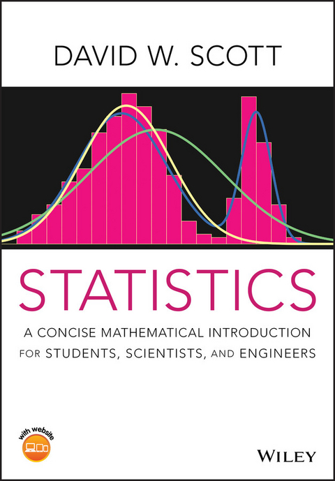
Statistics (eBook)

A Concise Mathematical Introduction for Students, Scientists, and Engineers

David W. Scott (Autor)

eBook Download: EPUB

2020
Wiley (Verlag)
978-1-119-67585-3 (ISBN)

Infos

Statistic: A Concise Mathematical Introduction for Students and Scientists offers a one academic term text that prepares the student to broaden their skills in statistics, probability and inference, prior to selecting their follow-on courses in their chosen fields, whether it be engineering, computer science, programming, data sciences, business or economics. 

The book places focus early on continuous measurements, as well as discrete random variables. By invoking simple and intuitive models and geometric probability, discrete and continuous experiments and probabilities are discussed throughout the book in a natural way. Classical probability, random variables, and inference are discussed, as well as material on understanding data and topics of special interest.

Topics discussed include:

•      Classical equally likely outcomes

•      Variety of models of discrete and continuous probability laws

•      Likelihood function and ratio

•      Inference

•      Bayesian statistics

With the growth in the volume of data generated in many disciplines that is enabling the growth in data science, companies now demand statistically literate scientists and this textbook is the answer, suited for undergraduates studying science or engineering, be it computer science, economics, life sciences, environmental, business, amongst many others. Basic knowledge of bivariate calculus, R language, Matematica and JMP is useful, however there is an accompanying website including sample R and Mathematica code to help instructors and students.

DAVID W. SCOTT is the Noah Harding Professor of Statistics at Rice University in Houston, Texas. He is a Fellow of the ASA, IMS, AAAS, an elected member of the ISI and received the 2004 Army Wilks Award and the 2008 ASA Founder's Award. He was formerly the Editor of the Journal of Computational and Graphical Statistics and currently serves as Co-Editor of Wiley Interdisciplinary Reviews: Computational Statistics. He is also the author of Multivariate Density Estimation: Theory, Practice, and Visualization.

Textauszug

1
Data Analysis and Understanding

The field of statistics has a rich history that has become tightly integrated into the emerging field of data sciences. Collaboration with computer scientists, numerical analysts, and decision makers characterizes the field. The role of statistics and statisticians is to find actionable information in a noisy collection of data. Every field of academic endeavor encounters this problem: from the electrical engineer trying to find a signal in a noisy channel to an English professor trying to determine the authorship of a contested newly discovered manuscript.

There are two basic tasks for the statistician. First is to characterize the distribution of possible outcomes using a batch of representative data. An actuary may be asked to find a dollar loss for car accidents that is not exceeded 99.999% of the time. An economist may be asked to provide useful summaries of a collection of income data. The histogram is our primary tool here, an idea that did not appear until the 17th century; see Graunt (1662), who analyzed death records during height of the plague outbreak in Europe.

The second task is that of prediction. A bank may wish to understand how credit risk is related to other information that may be available. A mechanical engineer may wish to understand the risk inherent in a new design under extreme conditions. Methods for performing this task underlie many algorithms today, for example, translating foreign languages or image recognition.

The mathematical backbone of all of our statistical methods is probability theory. Thus we study the basics of probability theory and random variables in the first part of this course. Statistical methods and the basics of statistical decision theory form the core of the middle third of this course. Specific tests and data analysis approaches finish our study.

1.1 Exploring the Distribution of Data

Tukey (1977) introduced a number of data summaries in his book Exploratory Data Analysis. Many are based on quantiles or percentiles of the data vector. Percentiles are particular choices of the sorted data. The middlemost is the median, or the 50th percentile. As a measure of spread, Tukey focused on the distance from the 25th to the 75th percentiles, the so‐called interquartile range (IQR). A three‐point summary would list these percentiles. Instead Tukey popularized the box‐and‐whiskers plot, which is a five‐point summary. The additional two points are intended to capture 99% of the data. These are drawn at a distance of from the two quartiles. Any points outside these whiskers are plotted as potential outliers.

1.1.1 Pearson's Father–Son Height Data

We illustrate these ideas on a set of data collected by Karl Pearson over a century ago. He recorded the heights of fathers and an adult son. In the left frame in Figure 1.1, we display a box‐and‐whiskers plot of these data. We see that the sons are taller than their fathers by about an inch. There are also more potential outliers among the sons for some reason.

In the middle frame of Figure 1.1, we show Tukey's stem‐and‐leaf plot of the 1078 differences of the heights of each son and his father. The range of the data is and the first seven sorted values rounded to one decimal place are . Each data point is decomposed into a stem and a leaf digit. Thus has a stem of and a leaf of 0. The top line is actually , although it is too small to see. With so much data, each stem is broken into two lines to provide more detail. Thus the next two lines show a stem of but no leaves twice. The fourth line shows and the fifth line reads and so on. This figure was generated using the command ; R Core Team (2018). (The default has half as many stems.) Thus the stem‐and‐leaf plot shows the frequency count of points for each stem as character strings.

In the right frame of Figure 1.1, we show the frequency counts in a histogram. The histogram uses a parameter called the bin width to construct an equally spaced mesh . Then we count the number of points in each interval. These counts are displayed as a bar chart. (The histogram can use any anchor point, although 0 is a common choice.) For the histogram shown, the anchor point selected was 0, and was chosen using Scott's rule ; see Scott (1979). This rule is discussed in Section 9.1.4.1. The default choice in function hist is Sturges' rule, discussed in Section 9.1.4.3, which chooses 11 bins with (not shown).

The choice of is often considered a matter of convenience. The stem‐and‐leaf plot using one‐digit integer stems limits its choices. By way of contrast, any positive real number can be used in a histogram. In Figure 1.2, we show the histograms using by Scott's rule, as well as and . Loosely speaking, the histograms using are missing useful information, while the histograms using display spurious detail. We discuss strategies for finding the best choice of in Section 9.1. In any case, the histogram is a powerful tool for understanding the full distribution of data.

Figure 1.1 Displays of the father–son height data collected by Karl Pearson: (left) box‐and‐whiskers plot; (middle) stem‐and leaf plot; (right) histogram.

Figure 1.2 Histograms of the sons' heights (top row) and fathers' heights (bottom row) using three bin widths: , , from left to right; see text.

1.1.2 Lord Rayleigh's Data

In Exploratory Data Analysis, Tukey (1977) demonstrates the box‐and‐whiskers plot using the Lord Rayleigh data, which measure the weight of nitrogen gas obtained by various means; see Table 1.1. Discrepancies in the results led to his discovery of the element argon. Rayleigh made measurements from 1892 to 1894, with a mean of 2.30584 and a standard deviation of 0.00537. It is common to assume such measurements of a fundamental quantity are normally distributed. Multiple experiments are run and the results averaged in the presumption that a more accurate estimate will result.

Table 1.1 Lord Rayleigh's 24 measurements (sorted) of the weight of a sample of nitrogen. The first 10 came from chemical samples, while the last 14 came from pure air.

2.29816

2.29849

2.29869

2.29889

2.29890

2.29940

2.30054

2.30074

2.30143

2.30182

2.30956

2.30986

2.31001

2.31010

2.31010

2.31012

2.31017

2.31024

2.31024

2.31026

2.31027

2.31028

2.31035

2.31163

Figure 1.3 Displays of Lord Rayleigh's 24 measurements of the atomic weight of nitrogen gas. (Left) Histogram with four bins; (middle) a second histogram; (right) stem‐and‐leaf display using the command .

In the left frame of Figure 1.3, we display a histogram with four (carefully selected) bins. The histogram is shown on a density scale, rather than a frequency scale, so that the area of the shaded region is 1. We shall see in Problem 1 that this is accomplished by dividing the bin counts by .

The first histogram in Figure 1.3 hides the interesting structure contained in the small dataset. The second histogram and stem‐and‐leaf plot show the two clusters quite clearly. Charting of data before the 1900s was not common, and looking at a table of the data would typically not reveal this feature. It turned out that Lord Rayleigh had combined various sources of the gas with several purifying agents and extraction methods. The samples originating from “pure air” were “contaminated” with argon. For the discovery of argon, Lord Rayleigh was awarded the Nobel Prize in Physics in 1904.

1.1.3 Discussion

Finding structure in data is a primary goal of data science. Graphical methods are powerful approaches to discovering unexpected or hidden structure. Some of these methods are better suited to small datasets. In a multivariate statistics course, we will learn how to analyze data with more than one variable. Modern genetic datasets often result in more than variables!

1.2 Exploring Prediction Using Data

The second fundamental task of statistics is prediction. Data for this task are typically ordered pairs, . The goal is to predict the value of the variable using the corresponding value of the variable. For example, we might try to predict a son's height () knowing the father's height (). Or a bank contemplating a mortgage loan may use a person's credit score to predict the probability the person will default on the loan.

The initial step is to plot a scatter diagram of the data points in order to determine if there is a strong relationship between and . The relationship, if it exists, is linear or nonlinear. If knowledge of does not convey any information about the value of , then the scatter diagram will have no slope or trends, with values just scattered around their average.

1.2.1 Body and Brain Weights of Land Mammals

In the left...

Produkt-Details

• Erscheint lt. Verlag: 12.8.2020
• Sprache: englisch
• Themenwelt: Mathematik / Informatik ► Mathematik ► Statistik
• Themenwelt: Mathematik / Informatik ► Mathematik ► Wahrscheinlichkeit / Kombinatorik
• Schlagworte: Angewandte Wahrscheinlichkeitsrechnung u. Statistik • Applied Probability & Statistics • classical probability • critical region • Finanz- u. Wirtschaftsstatistik • Gaussian distribution • normal data • Normal distribution • null hypothesis • poisson events • probability distributions • r successes • shift model • Statistics • Statistics for Finance, Business & Economics • Statistik • Time • two-side hypothesis test • unknown variance • Variance
• ISBN-10: 1-119-67585-5 / 1119675855
• ISBN-13: 978-1-119-67585-3 / 9781119675853