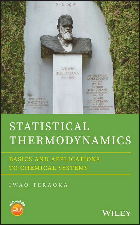
Statistical Thermodynamics (eBook)

Basics and Applications to Chemical Systems

Iwao Teraoka (Autor)

eBook Download: EPUB

2019
John Wiley & Sons (Verlag)
978-1-119-37528-9 (ISBN)

Infos

This textbook introduces chemistry and chemical engineering students to molecular descriptions of thermodynamics, chemical systems, and biomolecules.

• Equips students with the ability to apply the method to their own systems, as today's research is microscopic and molecular and articles are written in that language
• Provides ample illustrations and tables to describe rather difficult concepts
• Makes use of plots (charts) to help students understand the mathematics necessary for the contents
• Includes practice problems and answers

IWAO TERAOKA, PHD, is a professor of chemistry at Tandon School of Engineering of NYU. His current research areas include photonic sensors and liquid chromatography, but in early years he worked on physical chemistry of polymer solutions. He is a recipient of the 1994 NSF Young Investigator Award. Professor Teraoka is also the author of Polymer Solutions: An Introduction to Physical Properties and more than 100 original papers and 6 book chapters.

Textauszug

1
Introduction

Section 1.1 looks at the similarities and differences between classical thermodynamics and statistical thermodynamics. Then, in Section 1.2, we see several examples of phenomena that are beautifully described by statistical mechanics. Section 1.3 lists practices of notation adopted by this book.

1.1 Classical Thermodynamics and Statistical Thermodynamics

Classical thermodynamics, when applied to a closed system, starts with two fundamental laws. The first law of thermodynamics accounts for a balance of energy:

1.1

where the system receives heat d′Q and work d′W to change its internal energy by dU (see Figure 1.1). The prime in “d′” indicates that the quantity may not be a thermodynamic variable, i.e. not expressed as a total derivative. When the volume of the system changes from V to V + dV, d′W = −p dV, where p is the pressure.

Figure 1.1 A closed system received heat d′Q and work d′W from the surroundings to change its internal energy by dU.

The second law of thermodynamics expresses d′Q by a thermodynamic variable, but only when the change is reversible:

1.2

where T is the temperature. The second law introduces the entropy S.

In classical thermodynamics, we try to find relationships between macroscopic variables, S, T, U, V, and p. The equation of state is one of the relationships. We also learned different types of energy, specifically, enthalpy H, Helmholtz free energy F, and Gibbs free energy G. These measures of energy are convenient when we consider equilibria under different constraints. For example, at constant T and V, it is F that minimizes when the system is at equilibrium. Certainly, we can always maximize S of the universe (system + the surroundings), but knowing the details of the surroundings is not feasible or of our concern. Rather, we want to focus on the system, although it is the maximization of the entropy of the universe that dictates the equilibrium of the system. People have devised F for that purpose. If we minimize F of the system under given T and V, we are equivalently maximizing S of the universe. Likewise, G minimizes when the system's temperature and pressure are specified.

As you may recall, classical thermodynamics does not need to assume anything about the composition of the system – whether it is a gas or liquid, what molecules constitute the system, and so on. The system is a continuous medium; and it is uniform at all length scales, if it consists of a single phase. In other words, there are no molecules in this view.

Statistical thermodynamics, in contrast, starts with a molecule‐level description of the system – what types of molecules make up the system, whether interactions are present between molecules, and, if they are, how the interaction depends on the distance between molecules, and so on. Furthermore, statistical thermodynamics specifies microscopic states of the molecules, for example, their positions and velocities. If the molecules are monatomic, specifying the positions and velocities may be sufficient for our purposes. When the molecules are diatomic, however, we need to specify the states of rotation and vibration as well. If the molecule is polyatomic, specifying these states becomes more complicated. Even for a system of monatomic molecules, specifying the positions and velocities requires an astronomical number of variables. Typically, the number is close to Avogadro's number. Listing and evaluating all the variables is a daunting task. Fortunately, evaluating thermodynamics variables such as U, F, and G does not require all the details. It is rather the averages of the microscopic variables that count in evaluating the thermodynamic variables, and that is where statistical thermodynamics comes in.

1.2 Examples of Results Obtained from Statistical Thermodynamics

Here, we take a quick look at some of the results of applying statistical thermodynamics to different systems.

1.2.1 Heat Capacity of Gas of Diatomic Molecules

Figure 1.2 shows how the molar heat capacity CV/n of a gas consisting of diatomic molecules changes with temperature T. There are two characteristic temperatures Θrot and Θvib (rotation and vibration). Each diatomic molecule has its own Θrot and Θvib, and some of them are listed in Table 1.1.

Figure 1.2 Molar heat capacity CV/n of a gas consisting of diatomic molecules, plotted as a function of temperature T. At T around Θrot, the characteristic temperature of rotation, CV/n increases from 3∕₂R to 5∕₂R; and at around Θvib, the characteristic temperature of vibration, further increases to 7∕₂R.

Table 1.1 Characteristic temperature of rotation, Θrot, and characteristic temperature of vibration, Θvib, for some diatomic molecules.

Molecule

Θrot (K)

Θvib (K)

H2

87.6

6331

N2

2.88

3393

O2

2.08

2239

The molar heat capacity is 3∕₂R at T ≪ Θrot, where R is a gas constant. We see this range only for H2; for other gases, the boiling point is above Θrot. As T increases and surpasses Θrot, CV/n increases to 5∕₂R. There is a broad range of temperature that gives a nearly constant value of CV/n before it increases to 7∕₂R as T exceeds Θvib. For most diatomic molecules that are gas at room temperature (), Θrot ≪ RT ≪ Θvib, and that is why a gas of diatomic molecules has CV/n = 5∕₂R.

1.2.2 Heat Capacity of a Solid

Figure 1.3 depicts the molar heat capacity CV/n of a molecular solid (nonionic), plotted as a function of temperature T. At low temperatures, CV/n ∼ T3, and increases to a plateau value of 3R as T increases. Vibration in a lattice (crystal) accounts for this heat capacity. Einstein attempted to explain the heat capacity in his 1905 paper [1]. His statistical model correctly predicted 3R, but not T3. It is Debye who explained the ∼ T3 dependence by improving the Einstein model [2].

Figure 1.3 Heat capacity CV of a molecular solid, plotted as a function of temperature T. At close to T = 0, CV ∼ T3. With an increasing T, CV approaches a plateau value of 3R.

1.2.3 Blackbody Radiation

Anything with a temperature T > 0 radiates. A blackbody is a perfect emitter of the radiation (light) and also a perfect absorber. The radiation has different wavelength components and is not visible unless the wavelength falls in the visible range, 450–750 nm. When the radiation intensity is plotted as a function of T, the curve peaks at some wavelength λpeak (see Figure 1.4). With an increasing T, λpeak moves to a shorter wavelength, and the peak intensity increases. Stars exhibit different colors, and it is due to temperature differences. The radiation from the sun peaks at around 500 nm (blue–green), since its surface temperature is around 5800 K. A red star has a lower temperature, and a white star (λpeak ≅ 300 nm) has a higher temperature.

Figure 1.4 Irradiance of a blackbody at different temperatures, per wavelength, is plotted as a function of wavelength λ. The temperature is indicated adjacent to the curve.

The λpeak decreases as ∼T−1 as T increases, which is called Wien's displacement law, discovered in 1893. The profile of the spectrum has tails at both ends. The long‐wavelength tail follows ∼λ−4, and short‐wavelength tail ∼e−const./λ. The long‐wavelength tail was explained using classical electromagnetism, but it could not explain the short‐wavelength tail, or the Wien's law. Max Planck proposed a photon hypothesis – light consists of energy particles called photons, each carrying energy reciprocally proportional to λ – in 1900 [3]. He succeeded in explaining the whole radiation spectrum.

1.2.4 Adsorption

This example is more chemical than are the preceding examples. When a clean surface (glass, graphite, etc.) is exposed to a vapor, some molecules adsorb onto the surface (Figure...

Produkt-Details

• Erscheint lt. Verlag: 14.2.2019
• Sprache: englisch
• Themenwelt: Mathematik / Informatik ► Mathematik ► Statistik
• Themenwelt: Naturwissenschaften ► Chemie ► Physikalische Chemie
• Themenwelt: Naturwissenschaften ► Physik / Astronomie ► Thermodynamik
• Schlagworte: applications of statistical thermodynamics: chemical systems applications • biochemistry and statistical mechanics • biology and statistical mechanics • chemical engineering • Chemical Engineering Fundamentals • chemical thermodynamics • Chemie • Chemische Verfahrenstechnik • Chemistry • chemistry and statistical mechanics • Computer Science • Engineering • Grundlagen der Chemischen Verfahrenstechnik • guide to statistical thermodynamics • Materials Science • Materialwissenschaften • Materialwissenschaften / Theorie, Modellierung u. Simulation • Physical Chemistry • Physikalische Chemie • probability theory and physics • Statistical Mechanics • statistical mechanics and macroscopic thermodynamics • statistical mechanics to different thermodynamic systems • Statistical Thermodynamics • statistical thermodynamics basics • statistical thermodynamics fundamentals • Statistische Thermodynamik • Theory, Modeling & Simulation • thermodynamics • Thermodynamik
• ISBN-10: 1-119-37528-2 / 1119375282
• ISBN-13: 978-1-119-37528-9 / 9781119375289