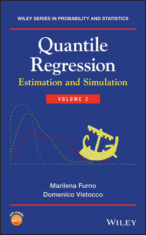
Quantile Regression (eBook)

Estimation and Simulation, Volume 2

Marilena Furno, Domenico Vistocco (Autoren)

eBook Download: EPUB

2018
John Wiley & Sons (Verlag)
978-1-118-86360-2 (ISBN)

Infos

Contains an overview of several technical topics of Quantile Regression 

Volume two of Quantile Regression offers an important guide for applied researchers that draws on the same example-based approach adopted for the first volume. The text explores topics including robustness, expectiles, m-quantile, decomposition, time series, elemental sets and linear programming. Graphical representations are widely used to visually introduce several issues, and to illustrate each method. All the topics are treated theoretically and using real data examples. Designed as a practical resource, the book is thorough without getting too technical about the statistical background.

The authors cover a wide range of QR models useful in several fields. The software commands in R and Stata are available in the appendixes and featured on the accompanying website. The text:

• Provides an overview of several technical topics such as robustness of quantile regressions, bootstrap and elemental sets, treatment effect estimators
• Compares quantile regression with alternative estimators like expectiles, M-estimators and M-quantiles
• Offers a general introduction to linear programming focusing on the simplex method as solving method for the quantile regression problem
• Considers time-series issues like non-stationarity, spurious regressions, cointegration, conditional heteroskedasticity via quantile regression
• Offers an analysis that is both theoretically and practical
• Presents real data examples and graphical representations to explain the technical issues

Written for researchers and students in the fields of statistics, economics, econometrics, social and environmental science, this text offers guide to the theory and application of quantile regression models.  

Marilena Furno, Department of Agriculture, University of Naples Federico II, Italy

Domenico Vistocco, Department of Economics and Law, University of Cassino, Italy

Textauszug

1
Robust regression

Introduction

This chapter considers the robustness of quantile regression with respect to outliers. A small sample model presented by Anscombe (1973) together with two real data examples are analyzed. The equations are estimated by OLS and by the median regression estimator, in order to compare their behavior in the presence of outliers. The impact of an outlying observation on a selected estimator can be measured by the influence function, and its sample approximation allows to evaluate the robustness of an estimator. The difference between the influence function of the OLS and of the quantile regression estimators is discussed, together with some other diagnostic measures defined to detect outliers.

1.1 The Anscombe data and OLS

In the linear regression model , the realizations of the variables and , in a sample of size with independent and identically distributed (i.i.d.) errors, allow to compute the unknown coefficients and . The ordinary least squares (OLS) estimator is the vector that minimizes the sum of squared errors, = ( ) . The minimization process yields the OLS estimators = and = , where and are the sample means. These estimators are the best linear unbiased (BLU) estimators, and OLS coincides with maximum likelihood in case of normally distributed errors. However OLS is not the sole criterion to compute the unknown vector of regression coefficients, and normality is not the unique error distribution. Other criteria are available, and they turn out to be very useful in the presence of outliers and when the errors are realization of non‐normal distributions. The small data set in Table 1.1 allows to explore some of the drawbacks of OLS that motivate the definition of different objective functions, that is different criteria defining the estimators of like in the quantile and the robust regression estimators.

Anscombe (1973) builds an artificial data set comprising observations of four dependent variables, , , , and , and two independent variables, and . This data set is reported in the first six columns of Table 1.1, while the remaining columns modify some observations of the original variables. The variables in the first six columns define four simple linear regression models where the OLS estimate of the intercept is always equal to and the OLS estimated slope is always equal to . These estimates are significantly different from zero, and the goodness of fit index is equal to in each of the four models. Figure 1.1 presents the plots of these models: the top‐left graph shows a regression model where OLS well summarizes the data set [ ]. In the other three models, however, the OLS estimates poorly describe the majority of the data in the sample.

In the top‐right graph, the data [ ] follow a non‐linear pattern, which is incorrectly estimated by a linear regression. Here the assumption of linearity is wrong, and the results are totally unreliable since the model is misspecified.

In the two bottom graphs, the OLS line is attracted by one anomalous value, that is by one observation that is far from the majority of the data. In the bottom‐left graph, the [ ] data set is characterized by one observation greater than all the others with respect to the dependent variable . This is a case of one anomalous observation in the dependent variable, reported in bold in the table, where the third observation presents the largest value of , the farthest from its median, , and from its mean . In this case the outlier attracts the OLS regression, causing a larger OLS estimated slope and a smaller OLS intercept. This example shows how one outlying observation can cause bias in the OLS estimates. If this observation is replaced by an observation closer to the rest of the data, for instance by the point ( ) as reported in the eighth column of the table, the variance of the dependent variable drops from of the original series to of the modified series, all the observations are on the same line, the goodness of fit index attains its maximum value, , and the unbiased OLS estimated coefficients are and . The results for the modified data set [ ] are depicted in the top‐right graph of Figure 1.2.

In the bottom‐right graph of Figure 1.1, instead, OLS computes a non‐existing proportionality between and . The proportionality between these two variables is driven by the presence of one outlying observation. In this case one observation, given by and reported in bold in the table, is an outlier in both dimensions, the dependent and the explanatory variable. If the eighth observation of is brought in line with all the other values of the dependent variable, that is if is replaced by as reported in the ninth column of Table 1.1, this observation is anomalous with respect to the independent variable alone. This case, for the data set [ ], is depicted in the bottom‐left graph of Figure 1.2. Even now there is no true link between the two variables; nevertheless OLS computes a non‐zero slope driven by the outlying value in . When the eighth observation is replaced by ( ) = (8.5 8), so that also the independent variable is brought in line with the rest of the sample, it becomes quite clear that does not depend on and that the previously estimated model is meaningless, as can be seen in the bottom‐right graph of Figure 1.2 for the data set [ ].

These examples show that there are different kinds of outliers: in the dependent variable, in the independent variable, or in both. The OLS estimator is attracted by these observations, and this causes a bias in the OLS estimated coefficients.

The bottom graphs of Figure 1.1 illustrate the impact of the so‐called leverage points, which are outliers generally located on one side of the scatterplot of the data. Their sideway position enhances the attraction, and thus the bias, of the OLS estimated line. The bias can be related to the definition of the OLS estimator, which is based on the sample mean of the variables. The mean is not a robust statistic, as it is highly influenced by anomalous values, and its lack of robustness is transmitted to the OLS estimator of the regression coefficients.

There are, however, cases of non‐influential outliers, i.e., of anomalous values that do not attract the OLS estimator and do not cause bias. This case is presented in the top‐left panel of Figure 1.2. In this graph the data set [ ] is modified to include one outlier in . In particular, by changing the fourth observation into – as reported in the seventh column of Table 1.1 – the estimated slope remains the same, , while the intercept increases to . The comparison of these OLS estimates is depicted in Figure 1.3: the lower line in this graph is estimated in the [ ] data set without outlier and yields the values and . The upper line is estimated in the modified data set [ ] with one outlier in the fourth observation of . The stability of the OLS slope in this example is linked to the location of the outlying point, which assumes a central position with respect to the explanatory variable, close to the mean of . Thus a non‐influential outlier is generally located at the center of the scatterplot and has an impact only on the intercept, without modifying the OLS slope.

The bias of the OLS estimator in the presence of influential outliers has prompted the definition of a wide class of estimators that, by curbing the impact of outliers, provide more reliable – robust – results. The payout of robust estimators is a reduced efficiency with respect to OLS in data sets without outlying observations. This is particularly true in case of normal error distributions, since under normality, OLS coincides with maximum likelihood and provides BLU estimators. However, in the presence of anomalous data, the idea of normally distributed errors must be discarded. Indeed the presence of outliers in a data set can be modeled by assuming non‐normal errors, like Student‐ , , double exponential, contaminated distributions, or any other distribution characterized by greater probability in the tails with respect to the normal case. A greater probability in the tails implies a greater probability of realizations far from the center of the distribution, that is, a greater probability of outliers in the data. Figure 1.4 compares the realizations of a Student‐ distribution with 2 degrees of freedom and a standard normal, represented by the dashed line, in a sample of observations. The realizations of the Student‐ distribution present a small peak in the left tail. This peak shows that data far from the center occur with a frequency greater than in the case of a normal density. Analogously, Figure 1.5 presents histogram of the realizations of a contaminated normal distribution . This distribution is defined as the linear combination of two normal distributions centered on the same mean, in this example centered on zero, but having different variances. The outliers are realizations of the distribution with higher variance. In Figure 1.5 a standard normal density, , generates 95% of the observations while the remaining 5% are realizations of , a contaminating normal distribution having zero mean and a larger standard error, . In this example the degree of contamination, i.e., the percentage of observations coming from the contaminating distribution , is 5%. In a sample of size , this...

Produkt-Details

• Erscheint lt. Verlag: 18.7.2018
• Reihe/Serie: Wiley Series in Probability and Statistics
• Reihe/Serie: Wiley Series in Probability and Statistics
• Reihe/Serie: Wiley Series in Probability and Statistics
• Sprache: englisch
• Themenwelt: Mathematik / Informatik ► Mathematik ► Statistik
• Themenwelt: Mathematik / Informatik ► Mathematik ► Wahrscheinlichkeit / Kombinatorik
• Schlagworte: Angewandte Wahrscheinlichkeitsrechnung u. Statistik • Applied Probability & Statistics • autoregressive models • Barrodale-Roberts algorithm for median and quantile regression • Bootstrap • Cointegration • Conditionally heteroskedastic models</p> • Contaminated errors • Correlation • dual plot • Elemental sets • Expectiles • Extremal quantiles • Finance & Investments • Financial Engineering • Finanztechnik • Finanz- u. Anlagewesen • Geometrical interpretation of the quantile regression problem • Inference in the unit root model • Influence function and diagnostic tools • Linear Programming • Linear programming formulation of the quantile regression problem • <p>Robust regression • m-estimators • M-quantiles • non-stationarity • Quantile regression process • Regression Analysis • Regressionsanalyse • Resampling and subsampling • Revised simplex algorithm • Simplex Algorithm • Spurious regression • Statistics • Statistik • Tests of changing coefficients • Treatment effect and decomposition
• ISBN-10: 1-118-86360-7 / 1118863607
• ISBN-13: 978-1-118-86360-2 / 9781118863602