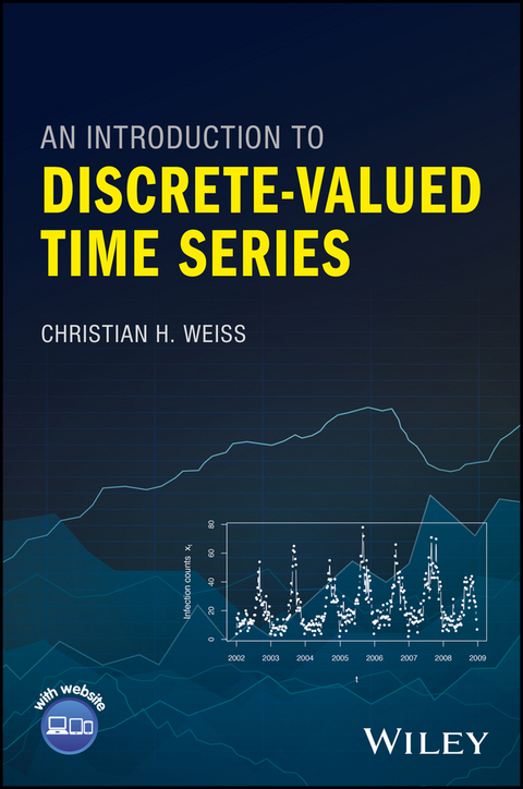
An Introduction to Discrete-Valued Time Series (eBook)

Christian H. Weiss (Autor)

eBook Download: EPUB

2017
John Wiley & Sons (Verlag)
978-1-119-09699-3 (ISBN)

Infos

A much-needed introduction to the field of discrete-valued time series, with a focus on count-data time series

Time series analysis is an essential tool in a wide array of fields, including business, economics, computer science, epidemiology, finance, manufacturing and meteorology, to name just a few. Despite growing interest in discrete-valued time series-especially those arising from counting specific objects or events at specified times-most books on time series give short shrift to that increasingly important subject area. This book seeks to rectify that state of affairs by providing a much needed introduction to discrete-valued time series, with particular focus on count-data time series.

The main focus of this book is on modeling. Throughout numerous examples are provided illustrating models currently used in discrete-valued time series applications. Statistical process control, including various control charts (such as cumulative sum control charts), and performance evaluation are treated at length. Classic approaches like ARMA models and the Box-Jenkins program are also featured with the basics of these approaches summarized in an Appendix. In addition, data examples, with all relevant R code, are available on a companion website.

• Provides a balanced presentation of theory and practice, exploring both categorical and integer-valued series
• Covers common models for time series of counts as well as for categorical time series,
• and works out their most important stochastic properties
• Addresses statistical approaches for analyzing discrete-valued time series and illustrates their implementation with numerous data examples
• Covers classical approaches such as ARMA models, Box-Jenkins program and how to generate functions
• Includes dataset examples with all necessary R code provided on a companion website

An Introduction to Discrete-Valued Time Series is a valuable working resource for researchers and practitioners in a broad range of fields, including statistics, data science, machine learning, and engineering. It will also be of interest to postgraduate students in statistics, mathematics and economics.

CHRISTIAN H. WEISS is a professor in the Department of Mathematics and Statistics, Helmut Schmidt University, Hamburg, Germany. His main area of research is discrete-valued time series. He has published numerous articles in this area and given lectures about time series analysis and discrete-valued time series. He has also written five lecture books in German.

Inhalt

Preface xi

About the CompanionWebsite xv

1 Introduction 1

Part I Count Time Series 9

2 A First Approach for Modeling Time Series of Counts: The

Thinning-based INAR(1)Model 11

2.0 Preliminaries: Notation and Characteristics of Count Distributions 11

2.1 The INAR(1) Model for Time-dependent Counts 16

2.1.1 Definition and Basic Properties 17

2.1.2 The Poisson INAR(1) Model 20

2.1.3 INAR(1) Models with More General Innovations 22

2.2 Approaches for Parameter Estimation 26

2.2.1 Method of Moments 26

2.2.2 Maximum Likelihood Estimation 28

2.3 Model Identification 29

2.4 Checking for Model Adequacy 32

2.5 A Real-data Example 34

2.6 Forecasting of INAR(1) Processes 37

3 Further Thinning-based Models for Count Time Series 43

3.1 Higher-order INARMA Models 43

3.2 Alternative Thinning Concepts 54

3.3 The Binomial AR Model 59

3.4 Multivariate INARMA Models 64

4 INGARCH Models for Count Time Series 73

4.1 Poisson Autoregression 73

4.2 Further Types of INGARCH Models 85

4.3 Multivariate INGARCH Models 93

5 Further Models for Count Time Series 95

5.1 Regression Models 95

5.2 Hidden-Markov Models 107

5.3 Discrete ARMA Models 116

Part II Categorical Time Series 119

6 Analyzing Categorical Time Series 121

6.1 Introduction to Categorical Time Series Analysis 122

6.2 Marginal Properties of Categorical Time Series 126

6.3 Serial Dependence of Categorical Time Series 128

7 Models for Categorical Time Series 133

7.1 Parsimoniously Parametrized Markov Models 133

7.2 Discrete ARMA Models 139

7.3 Hidden-Markov Models 146

7.4 Regression Models 151

Part III Monitoring Discrete-Valued Processes 161

8 Control Charts for Count Processes 163

8.1 Introduction to Statistical Process Control 163

8.2 Shewhart Charts for Count Processes 165

8.2.1 Shewhart Charts for i.i.d. Counts 166

8.2.2 Shewhart Charts for Markov-Dependent Counts 171

8.3 Advanced Control Charts for Count Processes 177

8.3.1 CUSUM Charts for i.i.d. Counts 178

8.3.2 CUSUM Charts for Markov-dependent Counts 182

8.3.3 EWMA Charts for Count Processes 186

9 Control Charts for Categorical Processes 193

9.1 Sample-based Monitoring of Categorical Processes 194

9.1.1 Sample-based Monitoring: Binary Case 194

9.1.2 Sample-based Monitoring: Categorical Case 198

9.2 Continuously Monitoring Categorical Processes 203

9.2.1 Continuous Monitoring: Binary Case 203

9.2.2 Continuous Monitoring: Categorical Case 209

Part IV Appendices 213

A Examples of Count Distributions 215

A.1 Count Models for an Infinite Range 215

A.2 Count Models for a Finite Range 221

A.3 Multivariate Count Models 223

B Basics about Stochastic Processes and Time Series 229

B.1 Stochastic Processes: Basic Terms and Concepts 229

B.2 Discrete-Valued Markov Chains 233

B.2.1 Basic Terms and Concepts 233

B.2.2 Stationary Markov Chains 236

B.3 ARMA Models: Definition and Properties 238

B.4 Further Selected Models for Continuous-valued Time Series 243

B.4.1 GARCH Models 243

B.4.2 VARMA Models 245

C Computational Aspects 249

C.1 Some Comments about the Use of R 250

C.2 List of R Codes 253

C.3 List of Datasets 256

References 257

List of Acronyms 275

List of Notations 277

Index 279

Textauszug

Chapter 1
Introduction

A (discrete-time) time series is a set of observations , which are recorded at times stemming from a discrete and linearly ordered set . An example of such a time series is plotted in Figure 1.1. This is the annual number of lynx fur returns for the MacKenzie River district in north-west Canada. The source is the Hudson's Bay Company, 1821–1934; see Elton & Nicholson (1942). These lynx data are discussed in many textbooks about time series analysis, to illustrate that real time series may exhibit quite complex seasonal patterns. Another famous example from the time series literature is the passenger data of Box & Jenkins (1970), which gives the monthly totals of international airline passengers (in thousands) for the period 1949–1960. These data (see Figure 1.2 for a plot) are often used to demonstrate the possible need for variance-stabilizing transformations.

Figure 1.1 Annual number of lynx fur returns (1821–1934); see Elton & Nicholson (1942).

Figure 1.2 Monthly totals (in thousands) of international airline passengers (1949–1960); see Box & Jenkins (1970).

Looking at the date of origin of the lynx data, it becomes clear that people have long been interested in data collected sequentially in time; see also the historical examples of time series in the books by Klein (1997) and Aigner et al. (2011). But even basic methods of analyzing such time series, as taught in any time series course these days, are rather new, mainly stemming from the last century. As shown by Klein (1997), the classical decomposition of time series into a trend component, a seasonal component and an “irregular component” was mostly developed in the first quarter of the 20th century. The periodogram, nowadays a standard tool to uncover seasonality, dates back to the work of A. Schuster in 1906. The (probably) first correlogram – a plot of the sample autocorrelation function against increasing time lag – can be found in a paper by G. U. Yule from 1926.

The understanding of the time series as stemming from an underlying stochastic process , and the irregular component from a stationary one, evolved around that time too (Klein, 1997), enabling an inductive analysis of time series. Here, is a sequence of random variables , where is a discrete and linearly ordered set with , while the observations are part of the realization of the process . Major early steps towards the modeling of such stochastic processes are A. N. Kolmogorov's extension theorem from 1933, the definitions of stationarity by A. Y. Khinchin and H. Wold in the 1930s, the development of the autoregressive (AR) model by G. U. Yule and G. T. Walker in the 1920s and 1930s, as well as of the moving-average (MA) model by G. U. Yule and E. E. Slutsky in the 1920s, their embedding into the class of linear processes by H. Wold in 1938, their combination to the full ARMA model by A. M. Walker in 1950, and, not to forget, the development of the concept of a Markov chain by A. Markov in 1906. All these approaches (see Appendix B for background information) are standard ingredients of modern courses on time series analysis, a fact which is largely due to G. E. P. Box and G. M. Jenkins and their pioneering textbook from 1970, in which they popularized the ARIMA models together with an iterative approach for fitting time series models, nowadays called the Box–Jenkins method. Further details on the history of time series analysis are provided in the books by Klein (1997) and Mills (2011), the history of ARMA models is sketched by Nie & Wu (2013), and more recent developments are covered by Tsay (2000) and Pevehouse & Brozek (2008).

From now on, let denote a time series stemming from the stochastic process ; to simplify notations, we shall later often use (full set of integers) or (set of non-negative integers). In the literature, we find several recent textbooks on time series analysis, for example the ones by Box et al. (2015), Brockwell & Davis (2016), Cryer & Chan (2008), Falk et al. (2012), Shumway & Stoffer (2011) amd Wei (2006). Typically, these textbooks assume that the random variables are continuously distributed, with the possible outcomes of the process being real numbers (the are assumed to have the range , where is the set of real numbers). The models and methods presented there are designed to deal with such real-valued processes.

In many applications, however, it is clear from the real context that the assumption of a continuous-valued range is not appropriate. A typical example is the one where the express a number of individuals or events at time , such that the outcome is necessarily integer-valued and hence discrete. If the realization of a random variable arises from counting, then we refer to it as a count random variable: a quantitative random variable having a range contained in the discrete set of non-negative integers. Accordingly, we refer to such a discrete-valued process as a count process, and to as a count time series. These are discussed in Part I of this book. Note that also the two initial data examples in Figures 1.1 and 1.2 are discrete-valued, consisting of counts observed in time. Since the range covered by these time series is quite large, they are usually treated (to a good approximation) as being real-valued. But if this range were small, as in the case of “low counts”, it would be misleading if ignoring the discreteness of the range.

An example of a low counts time series is shown in Figure 1.3, which gives the weekly number of active offshore drilling rigs in Alaska for the period 1990–1997; see Example 2.6.2 for further details. The time series consists of only a few different count values (between 0 and 6). It does not show an obvious trend or seasonal component, so the underlying process appears to be stationary. But it exhibits rather long runs of values that seem to be due to a strong degree of serial dependence. This is in contrast to the time series plotted in Figure 1.4, which concerns the weekly numbers of new infections with Legionnaires' disease in Germany for the period 2002–2008 (see Example 5.1.6). This has clear seasonal variations: a yearly pattern. Another example of a low counts time series with non-stationary behavior is provided by Figure 1.5, where the monthly number of “EA17” countries with stable prices (January 2000 to December 2006 in black, January 2007 to August 2012 in gray) is shown. As discussed in Example 3.3.4, there seems to be a structural change during 2007. If modeling such low counts time series, we need models that not only account for the discreteness of the range, but which are also able to deal with features of this kind. We shall address this topic in Part I of the present book.

Figure 1.3 Weekly counts of active offshore drilling rigs in Alaska (1990–1997), see Example 2.6.2.

Figure 1.4 Weekly counts of new infections with Legionnaires' disease in Germany (2002–2008); see Example 5.1.6.

Figure 1.5 Monthly counts of “EA17” countries with stable prices from January 2000 to August 2012; see Example 3.3.4.

All the data examples given above are count time series, which are the most common type of discrete-valued time series. But there is also another important subclass, namely categorical time series, as discussed in Part II of this book. For these, the outcomes stem from a qualitative range consisting of a finite number of categories. The particular case of only two categories is referred to as a binary time series. For the qualitative sleep status data shown in Figure 1.6, the six categories ‘qt’, …, ‘aw’ exhibit at least a natural ordering, so we are concerned with an ordinal time series. In other applications, not even such an inherent ordering exists (nominal time series). Then a time series plot such as the one in Figure 1.6 is no longer possible, and giving a visualization becomes much more demanding. In fact, the analysis and modeling of categorical time series cannot be done with the common textbook approaches, but requires tailor-made solutions; see Part II.

Figure 1.6 Successive EEG sleep states measured every minute; see Example 6.1.1.

For real-valued processes, autoregressive moving-average (ARMA) models are of central importance. With the (unobservable) innovations1 being independent and identically distributed (i.i.d.) random variables (white noise; see Example B.1.2 in Appendix B), the observation at time of such an ARMA process is defined as a weighted mean of past observations and innovations,

1.1

In other words, it is explained by a part of its own past as well as by an interaction of selected noise variables. Further details about ARMA models are summarized in Appendix B.3. Although these models themselves can be applied only to particular types of processes (stationary, short memory, and so on), they are at the core of several other models, such as those designed for non-stationary processes or processes with a long memory. In particular, the related generalized autoregressive conditional heteroskedasticity (GARCH) model, with its potential for application to financial time series, has become very popular...

Produkt-Details

• Erscheint lt. Verlag: 6.12.2017
• Sprache: englisch
• Themenwelt: Mathematik / Informatik ► Mathematik ► Statistik
• Themenwelt: Mathematik / Informatik ► Mathematik ► Wahrscheinlichkeit / Kombinatorik
• Schlagworte: ARMA discrete-valued time series models • Box-Jenkins discrete-valued time series program • categorical discrete-valued time series • categorical time series • classical approaches to modeling discrete-valued time series • count-data time series • count time series • discrete-valued time series • discrete-valued time series analysis • discrete-valued time series applications • discrete-valued time series data sets • discrete-valued time series data sets in R • discrete-valued time series examples • discrete-valued time series in computer science • discrete-valued time series in economics • discrete-valued time series in epidemiology • discrete-valued time series in finance • discrete-valued time series in meteorology • discrete-valued time series in traffic control • Econometric & Statistical Methods • Electrical & Electronics Engineering • Elektrotechnik u. Elektronik • integer discrete-valued time series • modeling discrete-valued time series • Ökonometrie • Ökonometrie u. statistische Methoden • Qualität u. Zuverlässigkeit • Quality & Reliability • statistical approaches to discrete-valued time series • Statistics • Statistik • Time Series • what is discrete-valued time series • Zeitreihe • Zeitreihen
• ISBN-10: 1-119-09699-5 / 1119096995
• ISBN-13: 978-1-119-09699-3 / 9781119096993