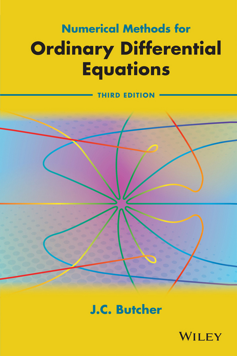
Numerical Methods for Ordinary Differential Equations (eBook)

J. C. Butcher (Autor)

eBook Download: EPUB

2016 | 3. Auflage
John Wiley & Sons (Verlag)
978-1-119-12152-7 (ISBN)

Infos

A new edition of this classic work, comprehensively revised to present exciting new developments in this important subject

The study of numerical methods for solving ordinary differential equations is constantly developing and regenerating, and this third edition of a popular classic volume, written by one of the world's leading experts in the field, presents an account of the subject which reflects both its historical and well-established place in computational science and its vital role as a cornerstone of modern applied mathematics.

In addition to serving as a broad and comprehensive study of numerical methods for initial value problems, this book contains a special emphasis on Runge-Kutta methods by the mathematician who transformed the subject into its modern form dating from his classic 1963 and 1972 papers.  A second feature is general linear methods which have now matured and grown from being a framework for a unified theory of a wide range of diverse numerical schemes to a source of new and practical algorithms in their own right.  As the founder of general linear method research, John Butcher has been a leading contributor to its development; his special role is reflected in the text.  The book is written in the lucid style characteristic of the author, and combines enlightening explanations with rigorous and precise analysis. In addition to these anticipated features, the book breaks new ground by including the latest results on the highly efficient G-symplectic methods which compete strongly with the well-known symplectic Runge-Kutta methods for long-term integration of conservative mechanical systems.

This third edition of Numerical Methods for Ordinary Differential Equations will serve as a key text for senior undergraduate and graduate courses in numerical analysis, and is an essential resource for research workers in applied mathematics, physics and engineering.

 

 

 

J.C Butcher, Emeritus Professor, University of Auckland, New Zealand

Textauszug

Chapter 1
Differential and Difference Equations

10 Differential Equation Problems

100 Introduction to differential equations

As essential tools in scientific modelling, differential equations are familiar to every educated person. In this introductory discussion we do not attempt to restate what is already known, but rather to express commonly understood ideas in the style that will be used for the rest of this book.

The aim will always be to understand, as much as possible, what we expect to happen to a quantity that satisfies a differential equation. At the most obvious level, this means predicting the value this quantity will have at some future time. However, we are also interested in more general questions such as the adherence to possible conservation laws or perhaps stability of the long-term solution. Since we emphasize numerical methods, we often discuss problems with known solutions mainly to illustrate qualitative and numerical behaviour.

Even though we sometimes refer to ‘time’ as the independent variable, that is, as the variable on which the value of the ‘solution’ depends, there is no reason for insisting on this interpretation. However, we generally use x to denote the ‘independent’ or ‘time’ variable and y to denote the ‘dependent variable’. Hence, differential equations will typically be written in the form

(100a)

where

Sometimes, for convenience, we omit the x in .

The terminology used in (100a) is misleadingly simple, because y could be a vector-valued function. Thus, if we are working in , and x is permitted to take on any real value, then the domain and range of the function f which defines a differential equation and the solution to this equation are given by

Since we might be interested in time values that lie only in some interval , we sometimes consider problems in which , and . When dealing with specific problems, it is often convenient to focus, not on the vector-valued functions f and y, but on individual components. Thus, instead of writing a differential equation system in the form of (100a), we can write coupled equations for the individual components:

(100b)

Autonomous differential equations

A differential equation for which f is a function not of x, but of y only, is said to be ‘autonomous’. Some equations arising in physical modelling are more naturally expressed in one form or the other, but we emphasize that it is always possible to write a non-autonomous equation in an equivalent autonomous form. All we need to do to change the formulation is to introduce an additional component into the y vector, and ensure that this can always maintain the same value as x, by associating it with the differential equation . Thus, the modified system is

(100c)

A system of differential equations alone does not generally define a unique solution, and it is necessary to add to the formulation of the problem a number of additional conditions. These are either ‘boundary conditions’, if further information is given at two or more values of x, or ‘initial conditions’, if all components of y are specified at a single value of x.

Initial value problems

If the value of is given, then the pair of equations

is known as an ‘initial value problem’. Our main interest in this book is with exactly this problem, where the aim is to obtain approximate values of for specific values of x, usually with , corresponding to the prediction of the future states of a differential equation system.

Note that for an N-dimensional system, the individual components of an initial value vector need to be given specific values. Thus, we might write

When the problem is formally converted to autonomous form (100c), the value of must be identical to , otherwise the requirement that should always equal x would not be satisfied.

For many naturally occurring phenomena, the most appropriate form in which to express a differential equation is as a high order system. For example, an equation might be of the form

with initial values given for . Especially important in the modelling of the motion of physical systems subject to forces are equation systems of the form

(100d)

where the equations, though second order, do have the advantages of being autonomous and without occurring amongst the arguments of .

To write (100d) in what will become our standard first order system form, we can introduce additional components . The differential equation system (100d) can now be written as the first order system

101 The Kepler problem

The problems discussed in this section are selected from the enormous range of possible scientific applications. The first example problem describes the motion of a single planet about a heavy sun. By this we mean that, although the sun exerts a gravitational attraction on the planet, we regard the corresponding attraction of the planet on the sun as negligible, and that the sun will be treated as being stationary. This approximation to the physical system can be interpreted in another way: even though both bodies are in motion about their centre of mass, the motion of the planet relative to the sun can be modelled using the simplification we have described. We also make a further assumption, that the motion of the planet is confined to a plane.

Let and denote rectangular coordinates centred at the sun, specifying at time x the position of the planet. Also let and denote the components of velocity in the and directions, respectively. If M denotes the mass of the sun, the gravitational constant and m the mass of the planet, then the attractive force on the planet will have magnitude

Resolving this force in the coordinate directions, we find that the components of acceleration of the planet, due to this attraction, are and , where the negative sign denotes the inward direction of the acceleration.

We can now write the equations of motion:

By adjusting the scales of the variables, the factor can be removed from the formulation, and we arrive at the equations

(101a)

(101b)

(101c)

(101d)

The solutions of this system are known to be conic sections, that is, ellipses, parabolas or hyperbolas, if we ignore the possibility that the trajectory is a straight line directed either towards or away from the sun. We investigate this further after we have shown that two ‘first integrals’, or invariants, of the solution exist.

Conservation of Hamiltonian and angular momentum

Theorem 101A

The quantities

are constant.

Proof

We verify that the values of and are zero if y satisfies (101a)–(101d). We have

and

The quantities H and A are the ‘Hamiltonian’ and ‘angular momentum’, respectively. Note that , where is the kinetic energy and is the potential energy.

A further property of this problem is its invariance under changes of scale of the variables:

The Hamiltonian and angular momentum get scaled to

Invariance under orthogonal transformations

A second type of transformation is based on a two-dimensional orthogonal transformation (that is, a rotation or a reflection or a composition of these) Q, where . The time variable x is invariant, and the position and velocity variables get transformed to

It is easy to see that implies that the trajectory lies entirely in a subspace defined by for some fixed angle . We move on from this simple case and assume that . The sign of H is of crucial importance: if then it is possible to obtain arbitrarily high values of without vanishing. We exclude this case for the present discussion and assume that . Scale H so that it has a value and at the same time A takes on a positive value. This value cannot exceed 1 because we can easily verify an identity involving the derivative of . This identity is

(101e)

Since the left-hand side cannot be negative, the quadratic function in r on the right-hand side must have real roots. This implies that . Write , for , where we see that e is the eccentricity of an ellipse on which the orbit lies. The minimum and maximum values of r are found to be and , respectively. Rotate axes so that when and . At this point we find that and . We will use these as initial values at .

Change to polar coordinates by writing . It is found that

so that, because , we find that

(101f)

From (101e) and (101f) we find a differential equation for the path traced out by the orbit

and we can verify that this is satisfied by

If we change back to Cartesian coordinates, we find that all points on the trajectory lie on the ellipse

with centre , eccentricity e, and major and minor axis lengths 1 and respectively.

As...

Produkt-Details

• Erscheint lt. Verlag: 5.8.2016
• Sprache: englisch
• Themenwelt: Mathematik / Informatik ► Mathematik ► Analysis
• Themenwelt: Technik
• Schlagworte: Applied Mathematics in Science • B-series • differential equation • General linear methods • Linear multistep • Mathematics • Mathematik • Mathematik in den Naturwissenschaften • Numerical analysis • Numerical Methods • numerische Methoden • Order arrow • Order of accuracy • Runge-Kutta • stability • symplectic
• ISBN-10: 1-119-12152-3 / 1119121523
• ISBN-13: 978-1-119-12152-7 / 9781119121527