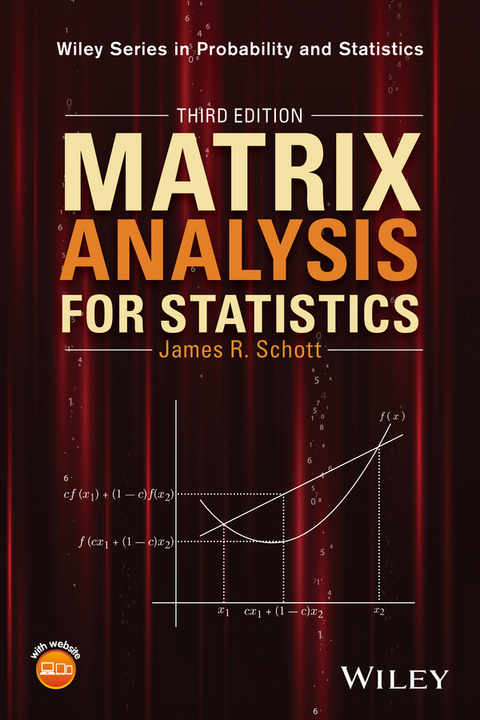
Matrix Analysis for Statistics (eBook)

James R. Schott (Autor)

eBook Download: EPUB

2016 | 3. Auflage
John Wiley & Sons (Verlag)
978-1-119-09246-9 (ISBN)

Infos

An up-to-date version of the complete, self-contained introduction to matrix analysis theory and practice

Providing accessible and in-depth coverage of the most common matrix methods now used in statistical applications, Matrix Analysis for Statistics, Third Edition features an easy-to-follow theorem/proof format. Featuring smooth transitions between topical coverage, the author carefully justifies the step-by-step process of the most common matrix methods now used in statistical applications, including eigenvalues and eigenvectors; the Moore-Penrose inverse; matrix differentiation; and the distribution of quadratic forms.

An ideal introduction to matrix analysis theory and practice, Matrix Analysis for Statistics, Third Edition features:

• New chapter or section coverage on inequalities, oblique projections, and antieigenvalues and antieigenvectors

• Additional problems and chapter-end practice exercises at the end of each chapter

• Extensive examples that are familiar and easy to understand

• Self-contained chapters for flexibility in topic choice

• Applications of matrix methods in least squares regression and the analyses of mean vectors and covariance matrices

Matrix Analysis for Statistics, Third Edition is an ideal textbook for upper-undergraduate and graduate-level courses on matrix methods, multivariate analysis, and linear models. The book is also an excellent reference for research professionals in applied statistics.

James R. Schott, PhD, is Professor in the Department of Statistics at the University of Central Florida. He has published numerous journal articles in the area of multivariate analysis. Dr. Schott's research interests include multivariate analysis, analysis of covariance and correlation matrices, and dimensionality reduction techniques.

James R. Schott, PhD, is Professor in the Department of Statistics at the University of Central Florida. He has published numerous journal articles in the area of multivariate analysis. Dr. Schott's research interests include multivariate analysis, analysis of covariance and correlation matrices, and dimensionality reduction techniques.

Textauszug

CHAPTER 1
A REVIEW OF ELEMENTARY MATRIX ALGEBRA

1.1 Introduction

In this chapter, we review some of the basic operations and fundamental properties involved in matrix algebra. In most cases, properties will be stated without proof, but in some cases, when instructive, proofs will be presented. We end the chapter with a brief discussion of random variables and random vectors, expected values of random variables, and some important distributions encountered elsewhere in the book.

1.2 Definitions and Notation

Except when stated otherwise, a scalar such as α will represent a real number. A matrix A of size m × n is the m × n rectangular array of scalars given by

and sometimes it is simply identified as . Sometimes it also will be convenient to refer to the th element of A, as ; that is, . If , then A is called a square matrix of order m, whereas A is referred to as a rectangular matrix when . An m × 1 matrix

is called a column vector or simply a vector. The element is referred to as the ith component of a. A matrix is called a row vector. The ith row and jth column of the matrix A will be denoted by and , respectively. We will usually use capital letters to represent matrices and lowercase bold letters for vectors.

The diagonal elements of the m × m matrix A are . If all other elements of A are equal to 0, A is called a diagonal matrix and can be identified as . If, in addition, for so that , then the matrix A is called the identity matrix of order m and will be written as or simply if the order is obvious. If and b is a scalar, then we will use to denote the diagonal matrix . For any m × m matrix A, will denote the diagonal matrix with diagonal elements equal to those of A, and for any m × 1 vector a, denotes the diagonal matrix with diagonal elements equal to the components of a; that is, and .

A triangular matrix is a square matrix that is either an upper triangular matrix or a lower triangular matrix. An upper triangular matrix is one that has all of its elements below the diagonal equal to 0, whereas a lower triangular matrix has all of its elements above the diagonal equal to 0. A strictly upper triangular matrix is an upper triangular matrix that has each of its diagonal elements equal to 0. A strictly lower triangular matrix is defined similarly.

The ith column of the m × m identity matrix will be denoted by ei; that is, ei is the m × 1 vector that has its ith component equal to 1 and all of its other components equal to 0. When the value of m is not obvious, we will make it more explicit by writing ei as . The m × m matrix whose only nonzero element is a 1 in the th position will be identified as .

The scalar zero is written 0, whereas a vector of zeros, called a null vector, will be denoted by 0 , and a matrix of zeros, called a null matrix, will be denoted by . The m × 1 vector having each component equal to 1 will be denoted by or simply 1 when the size of the vector is obvious.

1.3 Matrix Addition and Multiplication

The sum of two matrices A and B is defined if they have the same number of rows and the same number of columns; in this case,

The product of a scalar α and a matrix A is

The premultiplication of the matrix B by the matrix A is defined only if the number of columns of A equals the number of rows of B. Thus, if A is and B is , then will be the m × n matrix which has its th element, , given by

A similar definition exists for BA, the postmultiplication of B by A, if the number of columns of B equals the number of rows of A. When both products are defined, we will not have, in general, . If the matrix A is square, then the product AA, or simply , is defined. In this case, if we have , then A is said to be an idempotent matrix.

The following basic properties of matrix addition and multiplication in Theorem 1.1 are easy to verify.

Theorem 1.1

Let α and β be scalars and A, B, and C be matrices. Then, when the operations involved are defined, the following properties hold:

1. a. .
2. b. .
3. c. .
4. d. .
5. e. .
6. f. .
7. g. .
8. h. .

1.4 The Transpose

The transpose of an m × n matrix A is the n × m matrix obtained by interchanging the rows and columns of A. Thus, the th element of is . If A is and B is , then the th element of can be expressed as

Thus, evidently . This property along with some other results involving the transpose are summarized in Theorem 1.2.

Theorem 1.2

Let α and β be scalars and A and B be matrices. Then, when defined, the following properties hold:

1. a. .
2. b. .
3. c. .
4. d. .

If A is m × m, that is, A is a square matrix, then is also m × m. In this case, if , then A is called a symmetric matrix, whereas A is called a skew-symmetric if .

The transpose of a column vector is a row vector, and in some situations, we may write a matrix as a column vector times a row vector. For instance, the matrix defined in Section 1.2 can be expressed as . More generally, yields an m × n matrix having 1, as its only nonzero element, in the th position, and if A is an m × n matrix, then

1.5 The Trace

The trace is a function that is defined only on square matrices. If A is an m × m matrix, then the trace of A, denoted by , is defined to be the sum of the diagonal elements of A; that is,

Now if A is m × n and B is n × m, then AB is m × m and

This property of the trace, along with some others, is summarized in Theorem 1.3.

Theorem 1.3

Let α be a scalar and A and B be matrices. Then, when the appropriate operations are defined, we have the following properties:

1. a. .
2. b. .
3. c. .
4. d. .
5. e. if and only if .

1.6 The Determinant

The determinant is another function defined on square matrices. If A is an m × m matrix, then its determinant, denoted by , is given by

where the summation is taken over all permutations of the set of integers , and the function equals the number of transpositions necessary to change to an increasing sequence of components, that is, to . A transposition is the interchange of two of the integers. Although f is not unique, it is uniquely even or odd, so that is uniquely defined. Note that the determinant produces all products of m terms of the elements of the matrix A such that exactly one element is selected from each row and each column of A.

Using the formula for the determinant, we find that when . If A is 2×2, we have

and when A is 3×3, we get

The following properties of the determinant in Theorem 1.4 are fairly straightforward to verify using the definition of a determinant.

Theorem 1.4

If α is a scalar and A is an m × m matrix, then the following properties hold:

1. a. .
2. b. .
3. c. If A is a diagonal matrix, then .
4. d. If all elements of a row (or column) of A are zero, .
5. e. The interchange of two rows (or columns) of A changes the sign of .
6. f. If all elements of a row (or column) of A are multiplied by α, then the determinant is multiplied by α.
7. g. The determinant of A is unchanged when a multiple of one row (or column) is added to another row (or column).
8. h. If two rows (or columns) of A are proportional to one another, .

An alternative expression for can be given in terms of the cofactors of A. The minor of the element , denoted by , is the determinant of the matrix obtained after removing the ith row and jth column from A. The corresponding cofactor of , denoted by , is then given as .

Theorem 1.5

For any , the determinant of the m × m matrix A can be obtained by expanding along the ith row,

1.1

or expanding along the ith column,

1.2

Proof

We will just prove (1.1), as (1.2) can easily be obtained by applying (1.1) to . We...

Produkt-Details

• Erscheint lt. Verlag: 31.5.2016
• Reihe/Serie: Wiley Series in Probability and Statistics
• Reihe/Serie: Wiley Series in Probability and Statistics
• Reihe/Serie: Wiley Series in Probability and Statistics
• Sprache: englisch
• Themenwelt: Mathematik / Informatik ► Mathematik ► Statistik
• Themenwelt: Mathematik / Informatik ► Mathematik ► Wahrscheinlichkeit / Kombinatorik
• Themenwelt: Technik
• Schlagworte: Algebra • antieigenvalues • antieigenvectors • Applied Statistics • Inequalities • linear models • Mathematics • Mathematik • matrix analysis theory • matrix methods • multivariate analysis • oblique projections • Spezialthemen Statistik • Statistics • Statistics Special Topics • Statistics - Text & Reference • Statistik • Statistik / Lehr- u. Nachschlagewerke
• ISBN-10: 1-119-09246-9 / 1119092469
• ISBN-13: 978-1-119-09246-9 / 9781119092469