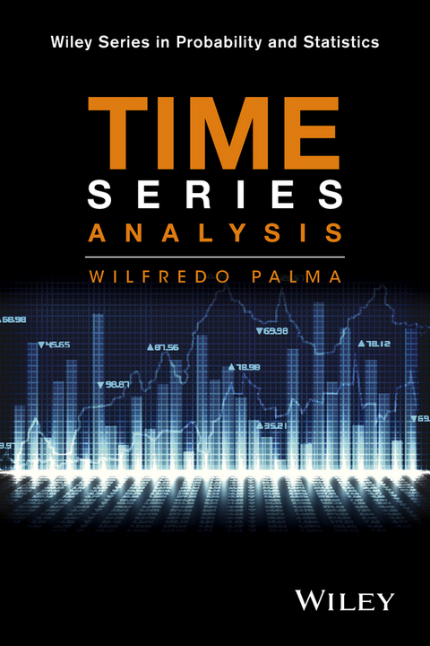
Time Series Analysis (eBook)

Wilfredo Palma (Autor)

eBook Download: EPUB

2016
John Wiley & Sons (Verlag)
978-1-118-63434-9 (ISBN)

Infos

A modern and accessible guide to the analysis of introductory time series data Featuring an organized and self-contained guide, Time Series Analysis provides a broad introduction to the most fundamental methodologies and techniques of time series analysis. The book focuses on the treatment of univariate time series by illustrating a number of well-known models such as ARMA and ARIMA. Providing contemporary coverage, the book features several useful and newlydeveloped techniques such as weak and strong dependence, Bayesian methods, non-Gaussian data, local stationarity, missing values and outliers, and threshold models. Time Series Analysis includes practical applications of time series methods throughout, as well as: Real-world examples and exercise sets that allow readers to practice the presented methods and techniques Numerous detailed analyses of computational aspects related to the implementation of methodologies including algorithm efficiency, arithmetic complexity, and process time End-of-chapter proposed problems and bibliographical notes to deepen readers knowledge of the presented material Appendices that contain details on fundamental concepts and select solutions of the problems implemented throughout A companion website with additional data fi les and computer codes Time Series Analysis is an excellent textbook for undergraduate and beginning graduate-level courses in time series as well as a supplement for students in advanced statistics, mathematics, economics, finance, engineering, and physics. The book is also a useful reference for researchers and practitioners in time series analysis, econometrics, and finance. Wilfredo Palma, PhD, is Professor of Statistics in the Department of Statistics at Pontificia Universidad Cat lica de Chile. He has published several refereed articles and has received over a dozen academic honors and awards. His research interests include time series analysis, prediction theory, state space systems, linear models, and econometrics. He is the author of Long-Memory Time Series: Theory and Methods, also published by Wiley.

Autor

Wilfredo Palma, PhD, is Professor of Statistics in the Department of Statistics at Pontificia Universidad Católica de Chile. Dr. Palma has published several refereed articles and has received over a dozen academic honors and awards. His research interests include time series analysis, prediction theory, state space systems, linear models, and econometrics. He is the author of Long-Memory Time Series: Theory and Methods, also published by Wiley.

Rezensionen

"This book offers a comprehensive overview of time series analysis...The focus throughout is on methodologies and techniques selected to help the reader develop a working knowledge of practical applications of time series methods... The author manages to incorporate a huge number of topics and his book verges on the encyclopedic...This is a book that would likely be of more use to a serious practitioner of time series analysis than anyone coming fresh to the subject." (Mathematical Association of America 29/03/2017)

"The book has many merits, covering carefully standard basic vocabulary of recently developing time series analysis and presenting lots of illustrative examples of applications that are well organized for the reader who intends to use R libraries for numerical computation" Yuzo Hosoya, MathSciNet, Aug 2017

Textauszug

Chapter 1
INTRODUCTION

A time series is a collection of observations taken sequentially in time. The nature of these observations can be as diverse as numbers, labels, colors, and many others. On the other hand, the times at which the observations were taken can be regularly or irregularly spaced. Moreover, time can be continuous or discrete. In this text, we focus primarily on describing methods for handling numeric time series observed at regular intervals of time. Note, however, that many nonnumeric data can be readily transformed to numeric. For instance, data concerning an election between candidate A and candidate B can be described by a numeric variable taking the value 0 for candidate A and 1 for candidate B. However, data observed at irregular time intervals are more difficult to handle. In this case, one may approximate the actual time to the closest integer value and still use the methodologies for handling regularly spaced series. If this approach does not provide adequate results, there are a number of more advanced techniques to treat those types of data. Another common problem in time series analysis is missing observations. In this case, the collected data display irregularly spaced observation times. There are special techniques for handling this problem and some of them are discussed in Chapter 11.

This introductory chapter presents a number of real-life time series data examples as well as provides a general overview of some essential concepts of the statistical analysis of time series, such as random variable, stochastic process, probability distribution and autocorrelation, among others. These notions are fundamental for the statistical modeling of serially dependent data.

Since this text attempts to reach a large audience interested in time series analysis, many of the more technical concepts are explained in a rigorous but simple manner. Readers interested in extending their knowledge of some particular concept in time series analysis will find an extensive list of references and a selected bibliographical discussion at the end of each chapter.

1.1 TIME SERIES DATA

Let us denote by {yt} a time series where t denotes the time at which the observation was taken. Usually, , where is the set of positive and negative integer values. In practice, however, only a finite stretch of data is available. In such situations, we can write the time series as {y1, y2, …, yn}. A time series {yt} corresponds to a stochastic process which in turn is composed of random variables observed across time. Both concepts are explained in detail later in this chapter.

Several examples of real-life time series data are presented in the following subsections. These data illustrations come from fields as diverse as, finance, economic, sociology, energy, medicine, climatology, and transport, among many others. Apart from exhibiting the time series, we describe their main features and some basic data transformations that help uncovering these characteristics.

1.1.1 Financial Data

Finance is a field where time series arises naturally from the evolution of indexes and prices. In what follows, we present two basic examples, the evolution of a well-known stock index and its volume of stock transactions.

Standard & Poor's Stock Index. Figure 1.1 shows the logarithm of the S&P500 daily stock index for the period from January 1950 to January 2014. Note that this index seems to increase with time, but there are some downward periods commonly denoted as bear markets. In order to study these indices, it is customary in finance to consider the logarithm return, which is defined as

where Pt denotes the price or the index value at time t. These returns are displayed in Figure 1.2. Observe the great drop in returns experienced on October 1987 and the abrupt changes or great volatility during 2009.

Figure 1.1 S&P500 daily stock log index, January 1950 to January 2014.

Figure 1.2 S&P500 daily log returns, January 1950 to January 2014.

Another look at the volatility is shown in Figure 1.3 where the squared returns, , are plotted. From this graph, the high volatility of this stock index is evident during these periods.

Figure 1.3 S&P500 daily square log returns, January 1950 to January 2014.

Financial time series possess specific features, such as those indicated above. Consequently, Chapter 6 describes methodologies for handling this type of data. These time series can be analyzed by means of the so-called conditionally heteroskedastic processes or stochastic volatility models, among others.

Volume of Transactions. As another example of financial data, the daily volume of transactions of the S&P500 stocks is displayed in Figure 1.4. Observe that this series exhibits an upward trend up to 2009.

Figure 1.4 S&P500 daily volume of transactions, January 1950 to January 2014.

On the other hand, Figure 1.5 depicts a logarithm transformation of the above time series. Note that the variance of the data across time is now more stabilized, emerging a seemingly overall upward trend, excepting the values after 2009 and some other periods.

Figure 1.5 S&P500 daily log volume of transactions, January 1950 to January 2014.

These transaction volume data can be considered as an example of a non-Gaussian time series. In particular, these observations are positive counts. Specific methods for modeling and predicting non-Gaussian data are described in Chapter 12.

1.1.2 Economic Data

Figure 1.6(a) exhibits the monthly US employment in the arts, entertainment and recreation section for the January 1990 to December 2012, measured in thousands of persons. On the other hand, Figure 1.6(b) shows the logarithm transformation of these data. Notice that this data transformation seems to stabilize the variance of the series across time. On both panels, however, a seasonal pattern and an upper trend are evident.

Figure 1.6 US employment arts, entertainment, and recreation, January 1990 to December 2012.

1.1.3 Hydrological Data

In hydrology, time series data is usually related to the collection of river flows observations though the years. For example, the yearly minimum water levels of the Nile river measured at the Roda gauge is a well-known time series exhibiting high levels of serial dependency. These measurements, available from Statlib, www.stat.cmu.edu, are displayed in Figure 1.7 spanning a time period from 622 A.D. to 1921 A.D.

Figure 1.7 Nile river yearly minimum level at the Roda gauge, from 622 A.D. to 1921 A.D.

Notice that there are several blocks of seemingly repeated values. That is, consecutive years having exactly the same minimum water level. Since the observations are specified by four digits, these repetitions are probably the result of a lack of new information. The analysis of this time series data also indicates that the first 100 observations seem to have a different serial dependence structure, suffering a structural break phenomenon.

A detailed analysis of this historically important hydrological time series is proved in Chapter 8, where the changes in the serial dependence structure of these observations are modeled. The analysis of these hydrological data was crucial in the formal study of the so-called long-memory processes reviewed in Chapter 2.

1.1.4 Air Pollution

Figure 1.8 exhibits a daily index that measures the particulate matter of diameter less than 2.5 μ in Santiago, Chile, for the period 1989–1999, commonly referred to as PM2.5. A log-transformed data is shown in Figure 1.9.

Figure 1.8 Air pollution data: daily PM2.5 measurements at Santiago, Chile, 1989 - 1999.

Figure 1.9 Air pollution data: log daily PM2.5 measurements at Santiago, Chile, 1989 - 1999.

These measurements indicate the level of air pollution in certain city or region. Note the seasonal behavior of this series, due to the effects of climate conditions across the year. In winter, the PM2.5 level increases dramatically. On the other hand, it appears that there is downward trend in the series, indicating an improvement of the air quality during that period. In order to stabilize the variance exhibited by this data, a logarithmic transformation has been made and the resulting series is shown in Figure 1.9. A possible downward trend is now more clear in the transformed data.

1.1.5 Transportation Data

Figure 1.10 shows the number of monthly passenger enplanements for the period from January 2004 to December 2013. These observations correspond to the number of passenger boarding an airplane in the United States in a given month. Note the seasonal behavior of this series derived from the annual cycle of winter and summer seasons. Besides, it seems that there was a drop on passenger enplanements around 2009, revealing a plausible effect of the financial crisis of that year. In this situation, it is possible that the process was affected by a structural break or structural change. Methodologies for...

Produkt-Details

• Erscheint lt. Verlag: 28.4.2016
• Reihe/Serie: Wiley Series in Probability and Statistics
• Reihe/Serie: Wiley Series in Probability and Statistics
• Reihe/Serie: Wiley Series in Probability and Statistics
• Sprache: englisch
• Themenwelt: Mathematik / Informatik ► Mathematik ► Statistik
• Themenwelt: Mathematik / Informatik ► Mathematik ► Wahrscheinlichkeit / Kombinatorik
• Themenwelt: Technik
• Schlagworte: business • data analytics • Econometrics • Economics • estimation methods • Finance • Finanz- u. Wirtschaftsstatistik • linear processes • <p>time series • non-Gaussian time series</p> • nonlinear time series • Nonstationary Processes • Ökonometrie • Prediction • Spectral Analysis • statistical modeling • Statistics • Statistics for Finance, Business & Economics • Statistik • Time Series • Time Series Analysis • Time Series Regression • Volkswirtschaftslehre • Zeitreihen • Zeitreihenanalyse
• ISBN-10: 1-118-63434-9 / 1118634349
• ISBN-13: 978-1-118-63434-9 / 9781118634349