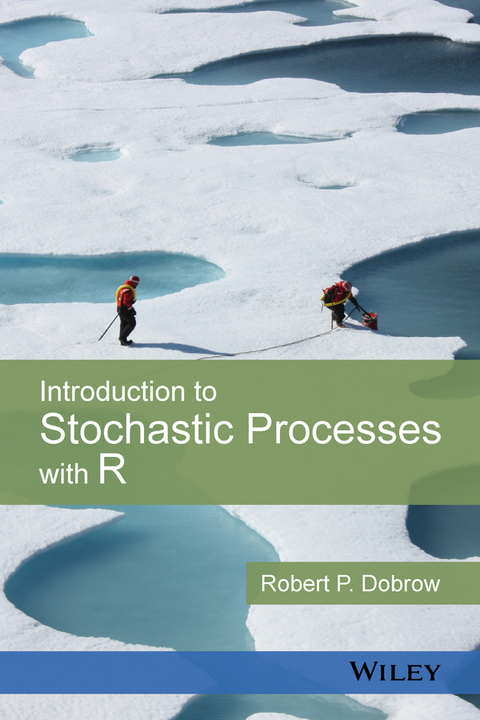
Introduction to Stochastic Processes with R (eBook)

Robert P. Dobrow (Autor)

eBook Download: EPUB

2016
John Wiley & Sons (Verlag)
978-1-118-74070-5 (ISBN)

Infos

An introduction to stochastic processes through the use of R

Introduction to Stochastic Processes with R is an accessible and well-balanced presentation of the theory of stochastic processes, with an emphasis on real-world applications of probability theory in the natural and social sciences. The use of simulation, by means of the popular statistical software R, makes theoretical results come alive with practical, hands-on demonstrations.

Written by a highly-qualified expert in the field, the author presents numerous examples from a wide array of disciplines, which are used to illustrate concepts and highlight computational and theoretical results. Developing readers' problem-solving skills and mathematical maturity, Introduction to Stochastic Processes with R features:

• More than 200 examples and 600 end-of-chapter exercises
• A tutorial for getting started with R, and appendices that contain review material in probability and matrix algebra
• Discussions of many timely and stimulating topics including Markov chain Monte Carlo, random walk on graphs, card shuffling, Black-Scholes options pricing, applications in biology and genetics, cryptography, martingales, and stochastic calculus
• Introductions to mathematics as needed in order to suit readers at many mathematical levels
• A companion web site that includes relevant data files as well as all R code and scripts used throughout the book

Introduction to Stochastic Processes with R is an ideal textbook for an introductory course in stochastic processes. The book is aimed at undergraduate and beginning graduate-level students in the science, technology, engineering, and mathematics disciplines. The book is also an excellent reference for applied mathematicians and statisticians who are interested in a review of the topic.

Robert P. Dobrow, PhD, is Professor of Mathematics and Statistics at Carleton College. He has taught probability and stochastic processes for over 15 years and has authored numerous research papers in Markov chains, probability theory and statistics.

Inhalt

Preface xi

Acknowledgments xv

List of Symbols and Notation xvii

About the Companion Website xxi

1 Introduction and Review 1

1.1 Deterministic and Stochastic Models 1

1.2 What is a Stochastic Process? 5

1.3 Monte Carlo Simulation 9

1.4 Conditional Probability 10

1.5 Conditional Expectation 18

Exercises 34

2 Markov Chains: First Steps 40

2.1 Introduction 40

2.2 Markov Chain Cornucopia 42

2.3 Basic Computations 52

2.4 Long-Term Behavior--the Numerical Evidence 59

2.5 Simulation 65

2.6 Mathematical Induction* 68

Exercises 70

3 Markov Chains for the Long Term 76

3.1 Limiting Distribution 76

3.2 Stationary Distribution 80

3.3 Can you Find the Way to State a? 94

3.4 Irreducible Markov Chains 103

3.5 Periodicity 106

3.6 Ergodic Markov Chains 109

3.7 Time Reversibility 114

3.8 Absorbing Chains 119

3.9 Regeneration and the Strong Markov Property* 133

3.10 Proofs of Limit Theorems* 135

Exercises 144

4 Branching Processes 158

4.1 Introduction 158

4.2 Mean Generation Size 160

4.3 Probability Generating Functions 164

4.4 Extinction is Forever 168

Exercises 175

5 Markov Chain Monte Carlo 181

5.1 Introduction 181

5.2 Metropolis-Hastings Algorithm 187

5.3 Gibbs Sampler 197

5.4 Perfect Sampling* 205

5.5 Rate of Convergence: the Eigenvalue Connection* 210

5.6 Card Shuffling and Total Variation Distance* 212

Exercises 219

6 Poisson Process 223

6.1 Introduction 223

6.2 Arrival, Interarrival Times 227

6.3 Infinitesimal Probabilities 234

6.4 Thinning, Superposition 238

6.5 Uniform Distribution 243

6.6 Spatial Poisson Process 249

6.7 Nonhomogeneous Poisson Process 253

6.8 Parting Paradox 255

Exercises 258

7 Continuous-Time Markov Chains 265

7.1 Introduction 265

7.2 Alarm Clocks and Transition Rates 270

7.3 Infinitesimal Generator 273

7.4 Long-Term Behavior 283

7.5 Time Reversibility 294

7.6 Queueing Theory 301

7.7 Poisson Subordination 306

Exercises 313

8 Brownian Motion 320

8.1 Introduction 320

8.2 Brownian Motion and Random Walk 326

8.3 Gaussian Process 330

8.4 Transformations and Properties 334

8.5 Variations and Applications 345

8.6 Martingales 356

Exercises 366

9 A Gentle Introduction to Stochastic Calculus* 372

9.1 Introduction 372

9.2 Ito Integral 378

9.3 Stochastic Differential Equations 385

Exercises 397

A Getting Started with R 400

B Probability Review 421

B.1 Discrete Random Variables 422

B.2 Joint Distribution 424

B.3 Continuous Random Variables 426

B.4 Common Probability Distributions 428

B.5 Limit Theorems 439

B.6 Moment-Generating Functions 440

C Summary of Common Probability Distributions 443

D Matrix Algebra Review 445

D.1 Basic Operations 445

D.2 Linear System 447

D.3 Matrix Multiplication 448

D.4 Diagonal, Identity Matrix, Polynomials 448

D.5 Transpose 449

D.6 Invertibility 449

D.7 Block Matrices 449

D.8 Linear Independence and Span 450

D.9 Basis 451

D.10 Vector Length 451

D.11 Orthogonality 452

D.12 Eigenvalue, Eigenvector 452

D.13 Diagonalization 453

Answers to Selected Odd-Numbered Exercises 455

References 470

Index 475

Rezensionen

"This text provides an excellent introduction to stochastic processes and their applications"...."Examples are plentiful and well chosen, and help to organize the material and to move it forward. Each section contains a good supply of exercises, both calculational and theoretical" Thomas Polaski, Mathematical Reviews, Sept 2017

Textauszug

CHAPTER 1
INTRODUCTION AND REVIEW

We demand rigidly defined areas of doubt and uncertainty!

–Douglas Adams, The Hitchhiker's Guide to the Galaxy

1.1 DETERMINISTIC AND STOCHASTIC MODELS

Probability theory, the mathematical science of uncertainty, plays an ever growing role in how we understand the world around us—whether it is the climate of the planet, the spread of an infectious disease, or the results of the latest news poll.

The word “stochastic” comes from the Greek stokhazesthai, which means to aim at, or guess at. A stochastic process, also called a random process, is simply one in which outcomes are uncertain. By contrast, in a deterministic system there is no randomness. In a deterministic system, the same output is always produced from a given input.

Functions and differential equations are typically used to describe deterministic processes. Random variables and probability distributions are the building blocks for stochastic systems.

Consider a simple exponential growth model. The number of bacteria that grows in a culture until its food source is exhausted exhibits exponential growth. A common deterministic growth model is to assert that the population of bacteria grows at a fixed rate, say 20% per minute. Let denote the number of bacteria present after minutes. As the growth rate is proportional to population size, the model is described by the differential equation

The equation is solved by the exponential function

where is the initial size of the population.

As the model is deterministic, bacteria growth is described by a function, and no randomness is involved. For instance, if there are four bacteria present initially, then after 15 minutes, the model asserts that the number of bacteria present is

The deterministic model does not address the uncertainty present in the reproduction rate of individual organisms. Such uncertainty can be captured by using a stochastic framework where the times until bacteria reproduce are modeled by random variables. A simple stochastic growth model is to assume that the times until individual bacteria reproduce are independent exponential random variables, in this case with rate parameter 0.20. In many biological processes, the exponential distribution is a common choice for modeling the times of births and deaths.

In the deterministic model, when the population size is , the number of bacteria increases by in 1 minute. Similarly, for the stochastic model, after bacteria arise the time until the next bacteria reproduces has an exponential probability distribution with rate per minute. (The stochastic process here is called a birth process, which is introduced in Chapter 7.)

While the outcome of a deterministic system is fixed, the outcome of a stochastic process is uncertain. See Figure 1.1 to compare the graph of the deterministic exponential growth function with several possible outcomes of the stochastic process.

Figure 1.1 Growth of a bacteria population. The deterministic exponential growth curve (dark line) is plotted against six realizations of the stochastic process.

The dynamics of a stochastic process are described by random variables and probability distributions. In the deterministic growth model, one can say with certainty how many bacteria are present after minutes. For the stochastic model, questions of interest might include:

• What is the average number of bacteria present at time ?
• What is the probability that the number of bacteria will exceed some threshold after minutes?
• What is the distribution of the time it takes for the number of bacteria to double in size?

In more sophisticated stochastic growth models, which allow for births and deaths, one might be interested in the likelihood that the population goes extinct, or reaches a long-term equilibrium.

In all cases, conclusions are framed using probability with the goal of quantifying the uncertainty in the system.

Example 1.1 PageRank

The power of internet search engines lies in their ability to respond to a user's query with an ordered list of web sites ranked by importance and relevance. The heart of Google's search engine is the PageRank algorithm, which assigns an importance value to each web page, called its page rank. The algorithm is remarkable given the massiveness of the web with over one trillion web pages, and is an impressive achievement of mathematics, particularly linear algebra.

Although the actual PageRank algorithm is complex with many technical (and secret) details, the page rank of a particular web page is easily described by means of a stochastic model. Consider a hypothetical web surfer who travels across the internet moving from page to page at random. When the surfer is on a particular web page, they pick one of the available hypertext links on that page uniformly at random and then move to that page.

The model can be described as a random walk by the web surfer on a giant graph called the webgraph. In the webgraph, vertices (nodes) are web pages. Vertex is joined to vertex by a directed edge if there is a hypertext link on page that leads to page . When the surfer is at vertex , they choose an edge leading away from uniformly at random from the set of available edges, and move to the vertex which that edge points to.

The random surfer model is an example of a more general stochastic process called random walk on a graph.

Imagine that the web surfer has been randomly walking across the web for a long, long time. What is the probability that the surfer will be at, say, page ? To make this more precise, let denote the probability that the surfer is at page after steps. The long-term probability of being at page is defined as .

This long-term probability is precisely the page rank of page . Intuitively, the long-term probability of being at a particular page will tend to be higher for pages with more incoming links and smaller for pages with few links, and is a measure of the importance, or popularity, of a page. The PageRank algorithm can be understood as an assignment of probabilities to each site on the web.

Figure 1.2 shows a simplified network of five pages. The numbers under each vertex label are the long-term probabilities of reaching that vertex, and thus the page rank assigned to that page.

Figure 1.2 Five-page webgraph. Vertex labels show long-term probabilities of reaching each page.

Many stochastic processes can be expressed as random walks on graphs in discrete time, or as the limit of such walks in continuous time. These models will play a central role in this book.

Example 1.2 Spread of infectious diseases

Models for the spread of infectious diseases and the development of epidemics are of interest to health scientists, epidemiologists, biologists, and public health officials. Stochastic models are relevant because of the randomness inherent in person-to-person contacts and population fluctuations.

The SIR (Susceptible–Infected–Removed) model is a basic framework, which has been applied to the spread of measles and other childhood diseases. At time , let represent the number of people susceptible to a disease, the number infected, and the number recovered and henceforth immune from infection. Individuals in the population transition from being susceptible to possibly infected to recovered .

The deterministic SIR model is derived by a system of three nonlinear differential equations, which model interactions and the rate of change in each subgroup.

A stochastic SIR model in discrete time was introduced in the 1920s by medical researchers Lowell Reed and Wade Frost from Johns Hopkins University. In the Reed–Frost model, when a susceptible individual comes in contact with someone who is infected there is a fixed probability that they will be infected.

Assume that each susceptible person is in contact with all those who are infected. Let be the probability that a susceptible individual is infected at time . This is equal to 1 minus the probability that the person is not infected at time , which occurs if they are not infected by any of the already infected persons, of which there are . This gives

Disease evolution is modeled in discrete time, where one time unit is the incubation period—also the recovery time—of the disease.

The model can be described with a coin-flipping analogy. To find , the number of individuals infected at time , flip coins (one for each susceptible), where the probability of heads for each coin is the infection probability . Then, the number of newly infected individuals is the number of coins that land heads.

The number of heads in independent coin flips with heads probability has a binomial distribution with parameters and . In other words, has a binomial distribution with and .

Having found the number of infected individuals at time , the number of susceptible persons decreases by the number of those infected. That is,

Although the Reed–Frost model is not easy to analyze exactly, it is straightforward to simulate on a computer. The graphs in Figure 1.3 were obtained by simulating the process assuming an initial population of 3 infected and 400 susceptible individuals, with individual infection probability . The number of those infected is plotted over 20 time units.

Figure...

Produkt-Details

• Erscheint lt. Verlag: 29.3.2016
• Sprache: englisch
• Themenwelt: Mathematik / Informatik ► Mathematik ► Statistik
• Themenwelt: Mathematik / Informatik ► Mathematik ► Wahrscheinlichkeit / Kombinatorik
• Themenwelt: Technik
• Schlagworte: Angewandte Wahrscheinlichkeitsrechnung u. Statistik • Applied Probability & Statistics • applied-statistics • business math • Differential • Functions • Gibbs sampler • Intro • Markov Chain • Martingales • mathematical equations • Metropolis Algorithm • Probability • Probability & Mathematical Statistics • Queueing Theory • random walks • Statistics • Statistik • stochastic-calculus • stochastic statistics • Wahrscheinlichkeitsrechnung • Wahrscheinlichkeitsrechnung u. mathematische Statistik • with R
• ISBN-10: 1-118-74070-X / 111874070X
• ISBN-13: 978-1-118-74070-5 / 9781118740705