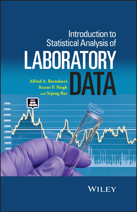
Introduction to Statistical Analysis of Laboratory Data (eBook)

Alfred Bartolucci, Karan P. Singh, Sejong Bae (Autoren)

eBook Download: EPUB

2015
John Wiley & Sons (Verlag)
978-1-119-08500-3 (ISBN)

Infos

Introduction to Statistical Analysis of Laboratory Data presents a detailed discussion of important statistical concepts and methods of data presentation and analysis

• Provides detailed discussions on statistical applications including a comprehensive package of statistical tools that are specific to the laboratory experiment process
• Introduces terminology used in many applications such as the interpretation of assay design and validation as well as 'fit for purpose' procedures including real world examples
• Includes a rigorous review of statistical quality control procedures in laboratory methodologies and influences on capabilities
• Presents methodologies used in the areas such as method comparison procedures, limit and bias detection, outlier analysis and detecting sources of variation
• Analysis of robustness and ruggedness including multivariate influences on response are introduced to account for controllable/uncontrollable laboratory conditions

Alfred A. Bartolucci is Professor Emeritus in the Department of Biostatistics, School of Public Health, University of Alabama at Birmingham. He has over 300 peer-reviewed publications (manuscripts and book chapters) in the areas of original statistical methodologic research and clinical and laboratory statistical applications. An endowed scholarship in Biostatistics at UAB was established in his honor.

Karan P. Singh is currently Professor of Medicine and serves as Director of the Biostatistics and Bioinformatics Shared Facility at the University of Alabama at Birmingham Comprehensive Cancer Center. He has authored or coauthored over 250 peer-reviewed articles, book chapters, and peer-reviewed congress or conference proceedings. He is a Fellow of the American Statistical association.

Sejong Bae is Professor of Medicine and serves as Co-Director of the Biostatistics and Bioinformatics Shared Facility; Deputy Director of the Coronary Artery Risk Development in Young Adults Coordination Center; and Director of Data, Information, and Statistics Core in the Division of Preventive Medicine. In 2009, he was elected to International Statistical Institute.

Inhalt

Descriptive Statistics

1.1 Measures of Central Tendency

1.2 Measures of Variation

1.3 Laboratory Example

1.4 Putting it All Together

1.5 Summary

Distributions and Hypothesis Testing in Formal Statistical Laboratory Procedures

2.1 Introduction

2.2 Confidence Intervals

2.3 Inferential Statistics - Hypothesis Testing

Method Validation

3.1 Introduction

3.2 Accuracy

3.4 Sensitivity, Specificity (Selectivity)

3.5 Method Validation and Method Agreement - Bland Altman

Methodologies in Outlier Analysis

4.1 Introduction

4.2 Some Outlier Determination Techniques

4.3. Combined Method Comparison Outlier Analysis

4.4 Some Consequences Of Outlier Removal

4.5 Considering Outlier Variance

Statistical Process Control

5.1 Introduction

5.2 Control Charts

5.3 Capability Analysis

5.4 Capability Analysis - An Alternate Consideration

Limits of Calibration

6.1 Calibration: Limit Strategies for Laboratory Assay Data

6.2 Limit Strategies

6.3 Method Detection Limits (EPA)

6.4 Data Near The Detection Limits

6.5 More on Statistical Management of Non Detects

6.6 The Kaplan-Meier Method (Non-Parametric Approach) for Analysis of Lab Data with Non-Detects

Calibration Bias

7. 1 Error

7.2 Uncertainty

7.3 Sources of Uncertainty

7.4 Estimation Methods of Uncertainty

7.5 Calibration Bias

7.6 Multiple Instruments

7.7 Crude vs. Precise Methodologies

Robustness and Ruggedness

8.1 Introduction

8.2 Robustness

8.3 uggedness

8.4 An Alternative Procedure for Ruggedness Determination

8.5 Ruggedness and System Suitability Tests

Rezensionen

"The book presents a detailed discussion of important statistical concepts and methods of data presentation and analysis.
-Provides detailed discussions on statistical applications including a comprehensive package of statistical tools that are specific to the laboratory experiment process.
- Introduces terminology used in many applications such as the interpretation of assay design and validation as well as fit for purpose" procedures including real world examples." (Zentralblatt MATH 2016)

Textauszug

Chapter 1
Descriptive Statistics

1.1 Measures of Central Tendency

One wishes to establish some basic understanding of statistical terms before we deal in detail with the laboratory applications. We want to be sure to understand the meaning of these concepts, since one often describes the data with which we are dealing in summary statistics. We discuss what is commonly known as measures of central tendency such as the mean, median, and mode plus other descriptive measures from data. We also want to understand the difference between samples and populations.

Data come from the samples we take from a population. To be specific, a population is a collection of data whose properties are analyzed. The population is the complete collection to be studied; it contains all possible data points of interest. A sample is a part of the population of interest, a subcollection selected from a population. For example, if one wanted to determine the preference of voters in the United States for a political candidate, then all registered voters in the United States would be the population. One would sample a subset, say, 5000, from that population and then determine from the sample the preference for that candidate, perhaps noting the percent of the sample that prefer that candidate over another. It would be impossible logistically and costwise in statistics to canvass the entire population, so we take what we believe to be a representative sample from the population. If the sampling is done appropriately, then we can generalize our results to the whole population. Thus, in statistics, we deal with the sample that we collect and make our decisions. Again, if we want to test a certain vegetable or fruit for food allergens or contaminants, we take a batch from the whole collection, send it to the laboratory and it is, thus, subjected to chemical testing for the presence or degree of the allergen or contaminants. There are certain safeguards taken when one samples. For example, we want the sample to appropriately represent the whole population. Factors relevant in considering the representativeness of a sample include the homogeneity of the food and the relative sizes of the samples to be taken, among other considerations. Therefore, keep in mind that when we do statistics, we always deal with the sample in the expectation that what we conclude generalizes to the whole population.

Now let's talk about what we mean when we say we have a distribution of the data. The following is a sample of size 16 of white blood cell (WBC) counts ×1000 from a diseased sample of laboratory animals:

Note that this data is purposely presented in ascending order. That may not necessarily be the order in which the data was collected. However, in order to get an idea of the range of the observations and have it presented in some meaningful way, it is presented as such. When we rank the data from the smallest to the largest, we call this a distribution.

One can see the distribution of the WBC counts by examining Figure 1.1. We'll use this figure as well as the data points presented to demonstrate some of the statistics that will be commonplace throughout the text. The height of the bars represents the frequency of counts for each of the values 5.13–6.8, and the actual counts are placed on top of the bars. Let us note some properties of this distribution. The mean is easy. It is obviously the average of the counts from 5.13 to 6.8 or . Algebraically, if we denote the elements of a sample of size as , then the sample mean in statistical notation is equal to

1.1

For example, in our aforementioned WBC data, , and so on, where .

Figure 1.1 Frequency Distribution of White Cell Counts

Then the mean is noted as earlier, .

The median is the middle data point of the distribution when there is an odd number of values and the average of the two middle values when there is an even number of values in the distribution. We demonstrate it as follows.

Note our data is:

The number of data points is an even number, or 16. Thus, the two middle values are in positions 8 and 9 underlined above. So the median is the average of 6.0 and 6.0 or .

Suppose we had a distribution of seven data points, which is an odd number, then the median is just the middle value or the value in position number 4. Note the following: . Thus, the median value is 5.7. The median is also referred to as the 50th percentile. Approximately 50% of the values are above it and 50% of the values are below it. It is truly the middle value of the distribution.

The mode is the most frequently occurring value in the distribution. If we examine our full data set of 16 points, one will note that the value 6.0 occurs four times. Also see Figure 1.1. Thus, the mode is 6.0. One can have a distribution with more than one mode. For example, if the values of 5.4 and 6.0 were each counted four times, then this would be a bimodal distribution or a distribution with two modes.

We have just discussed what is referred to as measures of central tendency. It is easy to see that the measures of central tendency from this data (mean, median, and mode) are all in the center of the distribution, and all other values are centered around them. In cases where the mean = median = mode as in our example, the distribution is seen to be symmetric. Such is not always the case.

Figure 1.2 deals with data that is skewed and not symmetric. Note the mode to the left indicating a high frequency of low values. These are potassium values from a laboratory sample. This data is said to be skewed to the right or positively skewed. We'll revisit this concept of skewness in Chapter 2 and later chapters as well. There are 23 values (not listed here) ranging from 30 to 250. One usually computes the geometric mean (GM) of the data of this form. Sometimes, GM is preferred to the arithmetic mean (ARM) since it is less sensitive to outliers or extreme values. Sometimes, it is called a “spread preserving” statistic. The GM is always less than or equal to the ARM and is commonly used with data that may be skewed and not normal or not symmetric, such as much laboratory data is not symmetric.

Figure 1.2 Frequency Distribution of Potassium Values

Suppose we have observations , then the GM is defined as

1.2

or equivalently

1.3

In our potassium example . Note that the ARM = 75.217.

1.2 Measures of Variation

We've learned some important measures of statistics. The mean, median, and mode describe some sample characteristics. However, they don't tell the whole story. We want to know more characteristics of the data with which we are dealing. One such measure is the dispersion or the variance. This particular measure has several forms in laboratory science and is essential to determining something about the precision of an experiment. We will discuss several forms of variance and relate them to data accordingly.

The range is the difference between the maximum and minimum value of the distribution. Referring to the WBC data:

Obviously, the range is easy to compute, but it only depends on the two most extreme values of the data. We want a value or measure of dispersion that utilizes all of the observations. Note the data in Table 1.1. For the sake of demonstration, we have three observations: 2, 4, and 9. These data are seen in the data column. Note their sum or total is 15. Their mean or average is 5. Note their deviation from the mean, 2 − 5 = −3, 4 − 5 = −1 and 9 − 5 = 4. The sum of their deviations is 0. This property is true for any size data set, that is, the sum of the deviations will be close to 0. This doesn't make much sense as a measure of dispersion or we would have a perfect world of no variation or dispersion of the data. The last column denoted as (Deviation)2 is the deviation column squared. And the sum of the squared deviations is 26.

Table 1.1 Demonstration of Variance

Observation

Data

Deviation

(Deviation)2

1

2

(2 − 5) = −3

(2 − 5)2 = 9

2

4

(4 − 5) = −1

(4 − 5)2 = 1

3

9

(9 − 5) = 4

(9 − 5)2 = 16

Sum

15

0

26

Average

5

0

26/(3 − 1) = 13

The variance of a sample is the average squared deviation from the sample mean. Specifically, from the previous sample of three values, . Thus, the variance is 13. Dividing by (3 − 1) = 2 instead of 3 gives us an unbiased estimator of the variance because it tends to closely estimate the true population variance. Note that if our sample size were 100, then dividing by 99 or 100 would not make much of a difference in the value of the variance. The adjustment of dividing the sum of squares of the deviation by the sample size minus 1, (n − 1), can be thought of as a small sample size adjustment. It allows us not to underestimate the variance but to conservatively overestimate...

Produkt-Details

• Erscheint lt. Verlag: 2.11.2015
• Sprache: englisch
• Themenwelt: Mathematik / Informatik ► Mathematik ► Angewandte Mathematik
• Themenwelt: Mathematik / Informatik ► Mathematik ► Statistik
• Themenwelt: Naturwissenschaften ► Chemie
• Themenwelt: Technik
• Schlagworte: Chemie • Chemistry • Drug QA/Analysis • laboratory statistics, method comparison, bioassay, validation, outliers, process control, calibration, detection limits, bias, robustness, ruggedness, system suitability • Qualitätssicherung • Qualitätssicherung / Analyse in der Pharmazie • Qualitätssicherung in der Chemie • Qualitätssicherung • Qualitätssicherung / Analyse in der Pharmazie • Qualitätssicherung in der Chemie • Quality assurance • Statistics • Statistik • Statistische Analyse
• ISBN-10: 1-119-08500-4 / 1119085004
• ISBN-13: 978-1-119-08500-3 / 9781119085003