Finite Mathematics (eBook)

Models and Applications

Carla C. Morris, Robert M. Stark (Autoren)

eBook Download: EPUB

2015
John Wiley & Sons (Verlag)
978-1-119-01538-3 (ISBN)

Infos

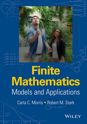
Features step-by-step examples based on actual data and connects fundamental mathematical modeling skills and decision making concepts to everyday applicability

Featuring key linear programming, matrix, and probability concepts, Finite Mathematics: Models and Applications emphasizes cross-disciplinary applications that relate mathematics to everyday life. The book provides a unique combination of practical mathematical applications to illustrate the wide use of mathematics in fields ranging from business, economics, finance, management, operations research, and the life and social sciences.

In order to emphasize the main concepts of each chapter, Finite Mathematics: Models and Applications features plentiful pedagogical elements throughout such as special exercises, end notes, hints, select solutions, biographies of key mathematicians, boxed key principles, a glossary of important terms and topics, and an overview of use of technology. The book encourages the modeling of linear programs and their solutions and uses common computer software programs such as LINDO. In addition to extensive chapters on probability and statistics, principles and applications of matrices are included as well as topics for enrichment such as the Monte Carlo method, game theory, kinship matrices, and dynamic programming.

Supplemented with online instructional support materials, the book features coverage including:

• Algebra Skills
• Mathematics of Finance
• Matrix Algebra
• Geometric Solutions
• Simplex Methods
• Application Models
• Set and Probability Relationships
• Random Variables and Probability Distributions
• Markov Chains
• Mathematical Statistics
• Enrichment in Finite Mathematics

An ideal textbook, Finite Mathematics: Models and Applications is intended for students in fields from entrepreneurial and economic to environmental and social science, including many in the arts and humanities.

Carla C. Morris, PhD, is Assistant Professor of Mathematics in the Associate in Arts Program at the University of Delaware. A member of The Institute for Operations Research and the Management Sciences and the Mathematical Association of America, Dr. Morris teaches courses ranging from college algebra to calculus and statistics.
Robert M. Stark, PhD, is Professor Emeritus in the Departments of Mathematical Sciences and Civil and Environmental Engineering at the University of Delaware. Dr. Stark's teaching and research interests include applied probability, mathematical optimization, operations research, and mathematics education.

Inhalt

Preface ix

About the Authors xi

1 Linear Equations and Mathematical Concepts 1

1.1 Solving Linear Equations 2

1.2 Equations of Lines and Their Graphs 7

1.3 Solving Systems of Linear Equations 15

1.4 The Numbers and e 21

1.5 Exponential and Logarithmic Functions 24

1.6 Variation 32

1.7 Unit Conversions and Dimensional Analysis 38

2 Mathematics of Finance 47

2.1 Simple and Compound Interest 47

2.2 Ordinary Annuity 55

2.3 Amortization 59

2.4 Arithmetic and Geometric Sequences 63

3 Matrix Algebra 71

3.1 Matrices 72

3.2 Matrix Notation, Arithmetic, and Augmented Matrices 78

3.3 Gauss-Jordan Elimination 89

3.4 Matrix Inversion and Input-Output Analysis 100

4 Linear Programming - Geometric Solutions 116

Introduction 116

4.1 Graphing Linear Inequalities 117

4.2 Graphing Systems of Linear Inequalities 121

4.3 Geometric Solutions to Linear Programs 125

5 Linear Programming - Simplex Method 136

5.1 The Standard Maximization Problem (SMP) 137

5.2 Tableaus and Pivot Operations 142

5.3 Optimal Solutions and the Simplex Method 149

5.4 Dual Programs 161

5.5 Non-SMP Linear Programs 167

6 Linear Programming - Application Models 182

7 Set and Probability Relationships 203

7.1 Sets 204

7.2 Venn Diagrams 210

7.3 Tree Diagrams 216

7.4 Combinatorics 221

7.5 Mathematical Probability 231

7.6 Bayes' Rule and Decision Trees 245

8 Random Variables and Probability Distributions 259

8.1 Random Variables 259

8.2 Bernoulli Trials and the Binomial Distribution 265

8.3 The Hypergeometric Distribution 273

8.4 The Poisson Distribution 279

9 Markov Chains 285

9.1 Transition Matrices and Diagrams 286

9.2 Transitions 291

9.3 Regular Markov Chains 295

9.4 Absorbing Markov Chains 304

10 Mathematical Statistics 314

10.1 Graphical Descriptions of Data 315

10.2 Measures of Central Tendency and Dispersion 323

10.3 The Uniform Distribution 331

10.4 The Normal Distribution 334

10.5 Normal Distribution Applications 348

10.6 Developing and Conducting a Survey 363

11 Enrichment in Finite Mathematics 371

11.1 Game Theory 372

11.2 Applications in Finance and Economics 385

11.3 Applications in Social and Life Sciences 394

11.4 Monte Carlo Method 403

11.5 Dynamic Programming 422

Answers to Odd Numbered Exercises 439

Using Technology 502

Glossary 506

Index 513

Rezensionen

"I would recommend this book to undergraduate students in mathematics, economics, engineering who are interested in fi nite mathematics." (Zentralblatt MATH, 2016)

Textauszug

Chapter 1
Linear Equations and Mathematical Concepts

1. 1.1 Solving Linear Equations
   1. 1. Example 1.1.1 Solving a Linear Equation
      2. Example 1.1.2 Solving for y
      3. Example 1.1.3 Simple Interest
      4. Example 1.1.4 Investment
      5. Example 1.1.5 Gasoline Prices
      6. Example 1.1.6 Breaking a Habit
2. 1.2 Equations of Lines and Their Graphs
   1. 1. Example 1.2.1 Ordered Pair Solutions
      2. Example 1.2.2 Intercepts and Graph of a Line
      3. Example 1.2.3 Slope-Intercept Form
      4. Example 1.2.4 Point-Slope Form
      5. Example 1.2.5 Temperature Conversion
      6. Example 1.2.6 Salvage Value
      7. Example 1.2.7 Parallel or Perpendicular Lines
3. 1.3 Solving Systems of Linear Equations
   1. 1. Example 1.3.1 Graphical Solutions to a System of Linear Equations
      2. Example 1.3.2 Substitution – Consistent System
      3. Example 1.3.3 Substitution–Inconsistent System
      4. Example 1.3.4 Elimination Method – Consistent System
      5. Example 1.3.5 Market Equilibrium
4. 1.4 The Numbers π and e
   1. The Number π
      1. Example 1.4.1 A Biblical π
   2. The Number e
5. 1.5 Exponential and Logarithmic Functions
   1. Exponential Functions
      1. Example 1.5.1 Using Laws of Exponents
      2. Example 1.5.2 Simplifying Exponential Equations
      3. Example 1.5.3 Simplifying Exponential Exponents
   2. Logarithmic Functions
      1. Example 1.5.4 Exponential and Logarithmic Forms
      2. Example 1.5.5 Simplifying Logarithms
      3. Example 1.5.6 Simplifying Logarithmic Expressions
      4. Example 1.5.7 Base 10 Exponents
      5. Example 1.5.8 Base e Exponents
6. 1.6 Variation
   1. 1. Example 1.6.1 Summer Wages
      2. Example 1.6.2 Hooke's Law
      3. Example 1.6.3 Geometric Similarity
      4. Example 1.6.4 Volume of a Sphere
      5. Example 1.6.5 Seawater Density
      6. Example 1.6.6 Illumination
      7. Example 1.6.7 Beam Strength
7. 1.7 Unit Conversions and Dimensional Analysis
   1. 1. Example 1.7.1 Dimensional Correctness
      2. Example 1.7.2 Speed Conversion
      3. Example 1.7.3 Time Conversion
      4. Example 1.7.4 Atoms of Nitrogen
      5. Example 1.7.5 Atoms of Hydrogen
8. Historical Notes and Comments

1.1 Solving Linear Equations

Mathematical descriptions, often as algebraic expressions, usually consist of alphanumeric characters and special symbols.

Physicists describe the distance, s, that an object falls under gravity in time, t, by . Here, the letters s and t are variables since their values may change, while, g, the acceleration of gravity is considered constant. While any letters can represent variables, typically the later letters of the alphabet are customary. The use of x and y is generic. Sometimes, it is convenient to use a letter that is descriptive of the variable, as t for time.

Earlier letters of the alphabet are customary for fixed values or constants. However, exceptions are widespread. The equal sign, a special symbol, is used to form an equation. An equation equates algebraic expressions. Numerical values for variables that preserve equality are called solutions to the equations.

For example, is an equation in a single variable, x. It is a conditional equation since it is only true when . Equations that hold for all values of the variable are called identities. For example, is an identity. By solving an equation, values of the variables that satisfy the equation are determined.

An equation in which only the first powers of variables appear is a linear equation. Every linear equation in a single variable can be solved using some or all of these properties:

1. Substitution – Substituting one expression for an equivalent one does not alter the original equation. For example, is equivalent to or .
2. Addition – Adding (or subtracting) a quantity to each side of an equation leaves it unchanged. For example, is equivalent to or .
3. Multiplication – Multiplying (or dividing) each side of an equation by a nonzero quantity leaves it unchanged. For example, is equivalent to or .

To Solve Single Variable Linear Equations

1. 1. Resolve fractions.
2. 2. Remove grouping symbols.
3. 3. Use addition and/or subtraction to move variable terms to one side of the equation.
4. 4. Divide the equation by the variable coefficient.
5. 5. Verify the solution in the original equation as a check.

 

Example 1.1.1 Solving a Linear Equation

Solve .

Solution:

To remove fractions, multiply both sides of the equation by 6, the least common denominator of 2 and 3. The revised equation becomes

Next, remove grouping symbols to yield

Now, subtract 4x and add 48 to both sides to yield

Finally, divide both sides by 5 (the coefficient of x) to attain . The result, is checked by substitution in the original equation:

Equations often contain more than one variable. To solve linear equations in several variables simply bring the variable of interest to one side. Proceed as for a single variable, considering the other variables as constants for the moment.

Example 1.1.2 Solving for y

Solve for y: .

Solution:

Move terms with y to one side of the equation and any remaining terms to the opposite side. Here, . Next, divide both sides by 4 to yield .

 

Example 1.1.3 Simple Interest

“Interest equals principal times rate times time” expresses the well-known simple interest formula, . Solve for time t.

Solution:

Clearly, and pr becomes the coefficient of t. Dividing by pr gives .

Mathematics is often called “the language of science” or “the universal language.” To study phenomena or situations of interest, mathematical expressions and equations are used to create a mathematical model. Extracting information from the mathematical model provides solutions and insights. These suggestions may aid in modeling skills.

To Solve Word Problems

1. 1. Read the problem carefully.
2. 2. Identify the quantity of interest and possibly useful formulas.
3. 3. A diagram may help.
4. 4. Assign symbols to variables and other unknown quantities.
5. 5. Translate words into an equation(s) using symbols for variables and unknowns.
6. 6. Solve for the quantity of interest.
7. 7. Check the solution and whether the proper question has been answered.

 

Example 1.1.4 Investment

Ms. Brown invests $5000 to yield 1% annual interest. What will she earn in 1 year?

Solution:

Here, the principal (original investment) is $5000. The interest rate is 0.01 (expressed as a decimal) and the time is 1 year.

Using the simple interest formula, , Ms. Brown's interest is

After 1 year, her capital becomes .

 

Example 1.1.5 Gasoline Prices

The June, 2014, East Coast regular grade gasoline average price (including tax) was about $3.64 per gallon. The comparable West Coast average was about $4.00 per gallon.

(a)What was the average regular grade gasoline price on the East Coast for 12 gallons of fuel?

(b)What was the average regular grade gasoline price on the West Coast for 25 gallons of fuel?

Solution:

1. a. On average, on the East Coast 12 gallons cost .
2. b. On average, on the West Coast 25 gallons cost .

 

♦ The famous yesteryear comedy team of Bud Abbott and Lou Costello used arithmetic shenanigans as the basis for many of their routines. The duo are probably best known for their “Who's on first” baseball routine. Google Ivars Peterson's “Math Trek” for some fun!

 

Example 1.1.6 Breaking a Habit

One theory for breaking an adverse habit (smoking, snacking, childish behavior, etc.) is to delay successive gratifications. Suppose a wait time of w hours before gratifying a desire. Next, an increment of v hours to hours to gratification. On the next occasion, the wait time is , and so on. Determine the wait time before gratification for the time.

Solution:

The first wait occurs at time w, the next v hours later so that the nth time is

Exercises 1.1

In Exercises 1–6 determine whether the equation is an identity, a conditional equation, or a contradiction.

1. 1.
2. 2....

Produkt-Details

• Erscheint lt. Verlag: 24.8.2015
• Sprache: englisch
• Themenwelt: Mathematik / Informatik ► Mathematik ► Allgemeines / Lexika
• Themenwelt: Technik
• Schlagworte: Algebra • Angewandte Mathematik • application models • Applied mathematics • Diskrete Mathematik • dynamic programing • finite Mathematics • Finite Mathematik • Game Theory • geometric solutions • kinship matrices • markov chains • Mathematical Modeling • Mathematical Statistics • Mathematics • mathematics of finance • Mathematik • Matrix Algebra • Monte Carlo Method • Probability & Mathematical Statistics • random variables and probability distributions • set and probability relationships • simplex methods • Statistics • Statistik • Wahrscheinlichkeitsrechnung u. mathematische Statistik
• ISBN-10: 1-119-01538-3 / 1119015383
• ISBN-13: 978-1-119-01538-3 / 9781119015383