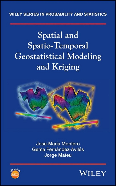
Spatial and Spatio-Temporal Geostatistical Modeling and Kriging (eBook)

José-María Montero, Gema Fernández-Avilés, Jorge Mateu (Autoren)

eBook Download: EPUB

2015
John Wiley & Sons (Verlag)
9781118762424 (ISBN)

Infos

Statistical Methods for Spatial and Spatio-Temporal Data Analysis provides a complete range of spatio-temporal covariance functions and discusses ways of constructing them. This book is a unified approach to modeling spatial and spatio-temporal data together with significant developments in statistical methodology with applications in R.

This book includes:

• Methods for selecting valid covariance functions from the empirical counterparts that overcome the existing limitations of the traditional methods.
• The most innovative developments in the different steps of the kriging process.
• An up-to-date account of strategies for dealing with data evolving in space and time.
• An accompanying website featuring R code and examples

José-María Montero and Gema Fernández-Avilés, Department of Statistics, University of Castilla-La Mancha, Spain

Jorge Mateu,  Department of Mathematics, University Jaume I of Castellon, Spain

Textauszug

List of figures

1.1	Location of the pollution monitoring stations in Madrid and map of predicted NOx levels (10 pm; average of the week days; 50th week of 2008) using geostatistical techniques.

1.2	Percentage of households with problems of pollution and odors in Madrid, Spain, 2001 (census tracts).

1.3	Fires in Castilla-La Mancha, Spain, 1998.

1.4	Location of the monitoring stations in the city of Madrid.

2.1	Simulation of a regionalized variable.

2.2	Four pairs of points separated by a distance h in a 2D domain.

2.3	Stationary and intrinsic hypotheses.

2.4	Top panel: Realization of a Wiener-Levy process. Bottom panel: First-order increments of the realization of the above Wiener-Levy process.

3.1	Spherical, exponential, and Gaussian covariance models with and different values of the scale parameter.

3.2	Spherical, exponential, and Gaussian models with and .

3.3	Bounded semivariogram and its covariogram counterpart.

3.4	Simulations of a rf having semivariograms that only differ in the range: (a) ; (b) ; (c) .

3.5	2D representation of simulations of two rf's with a semivariogram that only differs in the behavior near the origin: (a) linear, (b) parabolic.

3.6	Simulated fields of values using a semivariogram with scale parameter : (a) nugget effect = 0; (b) nugget effect = 0.25.

3.7	Nested semivariogram.

3.8	Upper panel: Spherical model. Left: . Right: . Middle panel: Simulation of a rf having a spherical semivariogram (2D representation). Left: . Right: . Bottom panel: Simulation of a rf having a spherical semivariogram (3D representation). Left: . Right: .

3.9	Left: Pure nugget semivariogram. Right: Simulation of a non-spatially correlated rf (2D representation).

3.10	Upper panel: Exponential model. Left: . Right: . Middle panel: Simulation of a rf having an exponential semivariogram (2D representation). Left: . Right: . Bottom panel: Simulation of a rf having an exponential semivariogram (3D representation). Left: . Right: .

3.11	Upper panel: Gaussian model. Left: . Right: . Middle panel: Simulation of a rf having a Gaussian semivariogram (2D representation). Left: . Right: . Bottom panel: Simulation of a rf having a Gaussian semivariogram (3D representation). Left: . Right: .

3.12	Cubic model with different ranges and the same sill ().

3.13	Simulation of a rf with cubic semivariogram model (3D representation). Left: . Right: .

3.14	Left: 3D representation of a simulation of a rf having a Gaussian semivariogram with . Right: 3D representation of a simulation of a rf having a cubic semivariogram with .

3.15

Upper panel, left: Stable model with the same sill () and scale parameter () but different shape parameter . Upper panel, right: 3D representation of a simulation of a rf having a stable semivariogram (). Bottom panel, left: 3D representation of a simulation of a rf having a stable semivariogram (). Bottom panel, right: 3D representation of a simulation of a rf having a stable semivariogram ().

3.16	Cauchy models with the same sill () and scale parameter () but different shape parameter .

3.17	K-Bessel model with the same scale parameter () and the same sill () but different shape parameter .

3.18	Cardinal sine models with the same sill () and different values of the scale parameter: (a) plot of the models; (b), (c) and (d) simulation of a rf having a cardinal sine model with , respectively (2D representation).

3.19	Power models.

3.20	Linear model.

3.21	Logarithmic model ().

3.22	Nested model composed of: (a) Pure nugget semivariogram (); (b) Spherical semivariogram (); (c) Spherical semivariogram (); (d) Nested semivariogram (3.40).

3.23	Tolerance region on .

3.24	Effect of the tolerance angle on a North-South empirical semivariogram. Tolerance angle: (a) , (b) , (c) , (d) . The observed regionalization was simulated with an spherical model ().

3.25	Twenty-five observed values in a grid.

3.26	Left: Empirical semivariogram (classic estimator). Right: Semivariogram cloud.

3.27	Observed values of logCO* at the 23 monitoring stations operating in Madrid, week 50, 10 pm. Left panel: 2D representation (black: higher values; white: lower values). Right panel: 3D representation.

3.28	Data on carbon monoxide in Madrid, week 50, 10 pm: (a) Classical empirical semivariogram; (b) Semivariogram cloud.

3.29	Observed points and data values.

3.30	Observed points and data values (without the outlier).

3.31	Left panel: Geometric anisotropy. Right panel: Zonal anisotropy.

3.32	Simulation of two rf's. Left panel: The geometric anisotropy case; Right panel: The zonal anisotropy case.

3.33	Simulation of a isotropic rf.

3.34	Semivariogram maps: (a) The isotropic case (circular contours); (b) The anisotropic case (elliptic contours, ). The axes depict lag distances in the corresponding coordinate system.

3.35	3D representation of zonal anisotropy. Left panel: Pure zonal anisotropy in vertical direction. Right panel: Directional semivariograms in horizontal directions (), vertical () and in an intermediate direction (). Source: Emery (2000, p. 111). Reproduced with permission of Xavier Emery.

3.36	Spherical models resulting from the automatic fitting (data on carbon monoxide in Madrid, week 50, 10 pm).

4.1	Location of eight observation points used for prediction at the non-observed point .

4.2	New location of the prediction point .

4.3	Prediction and prediction standard deviation (SD) maps of logCO*: January 2008, 2nd week, 10 am.

4.4	Prediction and prediction standard deviation (SD) maps of logCO*: January 2008, 2nd week, 3 pm.

4.5	Prediction and prediction standard deviation (SD) maps of logCO*: January 2008, 2nd week, 9 pm.

4.6	Six points, , discretizing the block V, and an observed point, .

4.7	Location of seven observation points used for prediction over the block .

4.8	Six points, discretizing , and six points, discretizing .

4.9	Coal-ash data. Location (reoriented) and observed values.

4.10	Coal-ash data. 3D scatterplot.

4.11	Contour plot of coal-ash percentages.

4.12	Coal-ash percentages surface interpolation (via triangulation).

4.13	Coal-ash percentages: Column and row summaries.

4.14	Prediction point.

4.15	Coal-ash percentages: Median-polish residuals.

4.16	Coal-ash data: Original data, median-polish drift and median-polish residuals (the lighter the color, the higher the value).

4.17	Coal-ash residuals: Classical semivariogram.

4.18	Exponential, spherical, cubic, and Gaussian models resulting from the WLS fitting. (Data on carbon monoxide in Madrid, week 50, 10 pm).

5.1	A spatio-temporal dataset on : 7 spatial locations observed at 3 moments in time (adapted from Luo 1998).

5.2	(a) Three...

Produkt-Details

• Erscheint lt. Verlag: 19.8.2015
• Reihe/Serie: Wiley Series in Probability and Statistics
• Reihe/Serie: Wiley Series in Probability and Statistics
• Reihe/Serie: Wiley Series in Probability and Statistics
• Sprache: englisch
• Themenwelt: Mathematik / Informatik ► Mathematik ► Angewandte Mathematik
• Themenwelt: Naturwissenschaften ► Biologie ► Ökologie / Naturschutz
• Themenwelt: Naturwissenschaften ► Geowissenschaften ► Geografie / Kartografie
• Themenwelt: Naturwissenschaften ► Geowissenschaften ► Geologie
• Themenwelt: Technik
• Schlagworte: biometrics • Biometrie • Environmental Modelling • environmental planning • Environmental Science • Environmental Statistics & Environmetrics • Environmental Studies • Functional geostatistics • Geostatistik • Kriging in space and space-time • Positive-Definite functions • Regionalized variables • Spatial Geostatistics • Spatio-temporal covariances • Spatio-temporal Geostatistics • Statistics • Statistik • Umweltforschung • Umweltstatistik • Umweltstatistik u. Environmetrics • Umweltwissenschaften • Univariate and Multivariate Geostatistics
• ISBN-13: 9781118762424 / 9781118762424