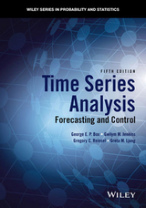
Time Series Analysis (eBook)

Forecasting and Control

George E. P. Box, Gwilym M. Jenkins, Gregory C. Reinsel, Greta M. Ljung (Autoren)

eBook Download: EPUB

2015 | 5. Auflage
John Wiley & Sons (Verlag)
978-1-118-67491-8 (ISBN)

Infos

Praise for the Fourth Edition

'The book follows faithfully the style of the original edition. The approach is heavily motivated by real-world time series, and by developing a complete approach to model building, estimation, forecasting and control.'
-Mathematical Reviews

Bridging classical models and modern topics, the Fifth Edition of Time Series Analysis: Forecasting and Control maintains a balanced presentation of the tools for modeling and analyzing time series. Also describing  the latest developments that have occurred in the field over the past decade through applications from areas such as business, finance, and engineering, the Fifth Edition continues to serve as one of the most influential and prominent works on the subject.

Time Series Analysis: Forecasting and Control, Fifth Edition provides a clearly written exploration of the key methods for building, classifying, testing, and analyzing stochastic models for time series and describes their use in five important areas of application: forecasting; determining the transfer function of a system; modeling the effects of intervention events; developing multivariate dynamic models; and designing simple control schemes.  Along with these classical uses, the new edition covers modern topics with new features that include:

• A redesigned chapter on multivariate time series analysis with an expanded treatment of Vector Autoregressive, or VAR models, along with a discussion of the analytical tools needed for modeling vector time series
• An expanded chapter on special topics covering  unit root testing,  time-varying volatility  models such as ARCH and GARCH, nonlinear time series models, and long memory models
• Numerous examples drawn from finance, economics, engineering, and other related fields
• The use of the publicly available R software for graphical illustrations and numerical calculations along with scripts that demonstrate the use of R for model building and forecasting
• Updates to literature references throughout and new end-of-chapter exercises
• Streamlined chapter introductions and revisions that update and enhance the exposition

Time Series Analysis: Forecasting and Control, Fifth Edition is a valuable real-world reference for researchers and practitioners in time series analysis, econometrics, finance, and related fields. The book is also an excellent textbook for beginning graduate-level courses in advanced statistics, mathematics, economics, finance, engineering, and physics.

The late George E. P. Box, PhD, was professor emeritus of statistics at the University of Wisconsin-Madison. He was a Fellow of the American Academy of Arts and Sciences and a recipient of the Samuel S. Wilks Memorial Medal of the American Statistical Association, the Shewhart Medal of the American Society for Quality, and the Guy Medal in Gold of the Royal Statistical Society. Dr. Box was also author of seven Wiley books.

The late Gwilym M. Jenkins, PhD, was professor of systems engineering at Lancaster University in the United Kingdom, where he was also founder and managing director of the International Systems Corporation of Lancaster. A Fellow of the Institute of Mathematical Statistics and the Institute of Statisticians, Dr. Jenkins had a prestigious career in both academia and consulting work that included positions at Imperial College London, Stanford University, Princeton University, and the University of Wisconsin-Madison. He was widely known for his work on time series analysis, most notably his groundbreaking work with Dr. Box on the Box-Jenkins models.

The late Gregory C. Reinsel, PhD, was professor and former chair of the department of Statistics at the University of Wisconsin-Madison. Dr. Reinsel's expertise was focused on time series analysis and its applications in areas as diverse as economics, ecology, engineering, and meteorology. He authored over seventy refereed articles and three books, and was a Fellow of both the American Statistical Association and the Institute of Mathematical Statistics.

Greta M. Ljung, PhD, is a statistical consultant residing in Lexington, MA. She received her doctorate from the University of Wisconsin-Madison where she did her research in time series analysis under the direction of Professor George Box. Dr. Ljung's career includes teaching positions at Boston University and Massachusetts Institute of Technology, and a position as Principal Scientist at AIR Worldwide in Boston. Her many accomplishments include joint work with George Box on a time series goodness of fit test, which is widely applied in econometrics and other fields.

Textauszug

1
Introduction

A time series is a sequence of observations taken sequentially in time. Many sets of data appear as time series: a monthly sequence of the quantity of goods shipped from a factory, a weekly series of the number of road accidents, daily rainfall amounts, hourly observations made on the yield of a chemical process, and so on. Examples of time series abound in such fields as economics, business, engineering, the natural sciences (especially geophysics and meteorology), and the social sciences. Examples of data of the kind that we will be concerned with are displayed as time series plots in Figures 2.1 and 4.1. An intrinsic feature of a time series is that, typically, adjacent observations are dependent. The nature of this dependence among observations of a time series is of considerable practical interest. Time series analysis is concerned with techniques for the analysis of this dependence. This requires the development of stochastic and dynamic models for time series data and the use of such models in important areas of application.

In the subsequent chapters of this book, we present methods for building, identifying, fitting, and checking models for time series and dynamic systems. The methods discussed are appropriate for discrete (sampled-data) systems, where observation of the system occurs at equally spaced intervals of time.

We illustrate the use of these time series and dynamic models in five important areas of application:

1. The forecasting of future values of a time series from current and past values.
2. The determination of the transfer function of a system subject to inertia—the determination of a dynamic input–output model that can show the effect on the output of a system of any given series of inputs.
3. The use of indicator input variables in transfer function models to represent and assess the effects of unusual intervention events on the behavior of a time series.
4. The examination of interrelationships among several related time series variables of interest and determination of appropriate multivariate dynamic models to represent these joint relationships among the variables over time.
5. The design of simple control schemes by means of which potential deviations of the system output from a desired target may, so far as possible, be compensated by adjustment of the input series values.

1.1 Five Important Practical Problems

1.1.1 Forecasting Time Series

The use at time t of available observations from a time series to forecast its value at some future time t + l can provide a basis for (1) economic and business planning, (2) production planning, (3) inventory and production control, and (4) control and optimization of industrial processes. As originally described by Holt et al. (1963), Brown (1962), and the Imperial Chemical Industries (ICI) monograph on short term forecasting (Coutie, 1964), forecasts are usually needed over a period known as the lead time, which varies with each problem. For example, the lead time in the inventory control problem was defined by Harrison (1965) as a period that begins when an order to replenish stock is placed with the factory and lasts until the order is delivered into stock.

We will assume that observations are available at discrete, equispaced intervals of time. For example, in a sales forecasting problem, the sales zt in the current month t and the sales zt−1, zt−2, zt−3, ... in previous months might be used to forecast sales for lead times l = 1, 2, 3, ..., 12 months ahead. Denote by zˆt(l) the forecast made at origin t of the sales zt+l at some future time t + l, that is, at lead time l. The function zˆt(l), which provides the forecasts at origin t for all future lead times, based on the available information from the current and previous values zt, zt−1, zt−2, zt−3, ... through time t, will be called the forecast function at origin t. Our objective is to obtain a forecast function such that the mean square of the deviations zt+l−zˆt(l) between the actual and forecasted values is as small as possible for each lead time l.

In addition to calculating the best forecasts, it is also necessary to specify their accuracy, so that, for example, the risks associated with decisions based upon the forecasts may be calculated. The accuracy of the forecasts may be expressed by calculating probability limits on either side of each forecast. These limits may be calculated for any convenient set of probabilities, for example, 50 and 95%. They are such that the realized value of the time series, when it eventually occurs, will be included within these limits with the stated probability. To illustrate, Figure 1.1 shows the last 20 values of a time series culminating at time t. Also shown are forecasts made from origin t for lead times l = 1, 2, ..., 13, together with the 50% probability limits.

Figure 1.1 Values of a time series with forecast function and 50% probability limits.

Methods for obtaining forecasts and estimating probability limits are discussed in detail in Chapter 5. These forecasting methods are developed based on the assumption that the time series zt follows a stochastic model of known form. Consequently, in Chapters 3 and 4 a useful class of such time series models that might be appropriate to represent the behavior of a series zt, called autoregressive integrated moving average (ARIMA) models, are introduced and many of their properties are studied. Subsequently, in Chapters 6, 7, and 8 the practical matter of how these models may be developed for actual time series data is explored, and the methods are described through the three-stage procedure of tentative model identification or specification, estimation of model parameters, and model checking and diagnostics.

1.1.2 Estimation of Transfer Functions

A topic of considerable industrial interest is the study of process dynamics discussed, for example, by Aström and Bohlin (1966, pp. 96–111) and Hutchinson and Shelton (1967). Such a study is made (1) to achieve better control of existing plants and (2) to improve the design of new plants. In particular, several methods have been proposed for estimating the transfer function of plant units from process records consisting of an input time series Xt and an output time series Yt. Sections of such records are shown in Figure 1.2, where the input Xt is the rate of air supply and the output Yt is the concentration of carbon dioxide produced in a furnace. The observations were made at 9-second intervals. A hypothetical impulse response function vj, j = 0, 1, 2, ..., which determines the transfer function for the system through a dynamic linear relationship between input Xt and output Yt of the form Yt=∑j=0∞vjXt−j, is also shown in the figure as a bar chart. Transfer function models that relate an input process Xt to an output process Yt are introduced in Chapter 11 and many of their properties are examined.

Figure 1.2 Input and output time series in relation to a dynamic system.

Methods for estimating transfer function models based on deterministic perturbations of the input, such as step, pulse, and sinusoidal changes, have not always been successful. This is because, for perturbations of a magnitude that are relevant and tolerable, the response of the system may be masked by uncontrollable disturbances referred to collectively as noise. Statistical methods for estimating transfer function models that make allowance for noise in the system are described in Chapter 12. The estimation of dynamic response is of considerable interest in economics, engineering, biology, and many other fields.

Another important application of transfer function models is in forecasting. If, for example, the dynamic relationship between two time series Yt and Xt can be determined, past values of both series may be used in forecasting Yt. In some situations, this approach can lead to a considerable reduction in the errors of the forecasts.

1.1.3 Analysis of Effects of Unusual Intervention Events to a System

In some situations, it may be known that certain exceptional external events, intervention events, could have affected the time series zt under study. Examples of such intervention events include the incorporation of new environmental regulations, economic policy changes, strikes, and special promotion campaigns. Under such circumstances, we may use transfer function models, as discussed in Section 1.1.2, to account for the effects of the intervention event on the series zt, but where the “input” series will be in the form of a simple indicator variable taking only the values 1 and 0 to indicate (qualitatively) the presence or absence of the event.

In these cases, the intervention analysis is undertaken to obtain a quantitative measure of the impact of the intervention event on the time series of interest. For example, Box and Tiao (1975) used...

Produkt-Details

• Erscheint lt. Verlag: 2.6.2015
• Reihe/Serie: Wiley Series in Probability and Statistics
• Reihe/Serie: Wiley Series in Probability and Statistics
• Reihe/Serie: Wiley Series in Probability and Statistics
• Sprache: englisch
• Themenwelt: Mathematik / Informatik ► Mathematik ► Statistik
• Themenwelt: Mathematik / Informatik ► Mathematik ► Wahrscheinlichkeit / Kombinatorik
• Themenwelt: Technik
• Schlagworte: Ökonometrie • ARIMA Models • Bayesian inference • business • Econometrics • econometrics</p> • Economics • Finance • Forecasting • Industrial Engineering • Industrial Engineering / Quality Control • Industrielle Verfahrenstechnik • <p>time series • Mathematics • Modeling • multivariate dynamic models • Ökonometrie • Qualitätssicherung • Qualitätssicherung i. d. Industriellen Verfahrenstechnik • Qualitätssicherung • Qualitätssicherung i. d. Industriellen Verfahrenstechnik • quality control • R software • seasonal adjustments • Statistics • Statistik • stochastic model • Time Series • VAR models • Volatility Models • Volkswirtschaftslehre • Zeitreihen • Zeitreihenanalyse
• ISBN-10: 1-118-67491-X / 111867491X
• ISBN-13: 978-1-118-67491-8 / 9781118674918