Understanding the Discrete Element Method (eBook)
John Wiley & Sons (Verlag)
978-1-118-56728-9 (ISBN)
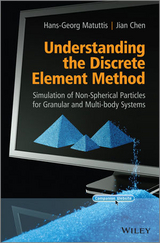
Gives readers a more thorough understanding of DEM and equips researchers for independent work and an ability to judge methods related to simulation of polygonal particles
- Introduces DEM from the fundamental concepts (theoretical mechanics and solidstate physics), with 2D and 3D simulation methods for polygonal particles
- Provides the fundamentals of coding discrete element method (DEM) requiring little advance knowledge of granular matter or numerical simulation
- Highlights the numerical tricks and pitfalls that are usually only realized after years of experience, with relevant simple experiments as applications
- Presents a logical approach starting withthe mechanical and physical bases,followed by a description of the techniques and finally their applications
- Written by a key author presenting ideas on how to model the dynamics of angular particles using polygons and polyhedral
- Accompanying website includes MATLAB-Programs providing the simulation code for two-dimensional polygons
Recommended for researchers and graduate students who deal with particle models in areas such as fluid dynamics, multi-body engineering, finite-element methods, the geosciences, and multi-scale physics.
Hans-Georg Matuttis, The University of Electro-Communications, Japan
Jian Chen, RIKEN Advanced Institute for Computational Science, Japan
Gives readers a more thorough understanding of DEM and equips researchers for independent work and an ability to judge methods related to simulation of polygonal particles Introduces DEM from the fundamental concepts (theoretical mechanics and solidstate physics), with 2D and 3D simulation methods for polygonal particles Provides the fundamentals of coding discrete element method (DEM) requiring little advance knowledge of granular matter or numerical simulation Highlights the numerical tricks and pitfalls that are usually only realized after years of experience, with relevant simple experiments as applications Presents a logical approach starting withthe mechanical and physical bases,followed by a description of the techniques and finally their applications Written by a key author presenting ideas on how to model the dynamics of angular particles using polygons and polyhedral Accompanying website includes MATLAB-Programs providing the simulation code for two-dimensional polygons Recommended for researchers and graduate students who deal with particle models in areas such as fluid dynamics, multi-body engineering, finite-element methods, the geosciences, and multi-scale physics.
Hans-Georg Matuttis, The University of Electro-Communications, Japan Jian Chen, RIKEN Advanced Institute for Computational Science, Japan
1
Mechanics
We start with an outline of classical mechanics, to provide a framework for the discrete element method (DEM). While most of the material in this chapter can be found scattered in various books on mechanics, no text seems to be available which covers concisely the concepts needed for DEM simulation. This chapter is intended as a crash course in theoretical mechanics, with an emphasis on issues relevant to computer implementation and testing. We give a list of secondary literature that the reader may refer to for further details.
1.1 Degrees of freedom
Before discussing the dynamics of a mechanical system, we need to understand the nature of the variables in the system. There are independent variables on the one hand, usually called ‘degrees of freedom’, and then there are dependent variables which depend on the degrees of freedom, via algebraic relations or derivatives.
1.1.1 Particle mechanics and constraints
The concept of a ‘mass point’ means that we neglect the size of the mass and are interested only in its trajectory. The position of a single mass point moving along the Cartesian x-axis is described by the value of x, which corresponds to a single degree of freedom. A point moving in the xy-plane has two degrees of freedom, r2D = (x, y), and a point moving in three-dimensional real space will have three degrees of freedom, r3D = (x, y, z). Although we can describe the motion of a point in three-dimensional space by four ‘space-time coordinates’ using the tuple (x, y, z, t), in classical mechanics t is not considered a degree of freedom but rather a parameter, i.e. an independent variable which cannot be influenced.
Two mass points moving independently along the x-axis represent two degrees of freedom, r1 and r2 (here and in the following, we assume equal masses). If we ‘glue’ these two particles together at distance d = r1 − r2 as in Figure 1.1, one degree of freedom gets lost, and we are left with only a single degree of freedom; in this case we can use either of r1, r2 or the average (r1+r2)/2 to determine the position of both particles uniquely. This means that one constraint between two position variables eliminates one degree of freedom.
Figure 1.1 In two dimensions, the number of degrees of freedom ndof for 1, 2, 3 or 4 constrained particles with an increasing number of constraints introduced. Newly added constraints are in black; previous constraints are in gray.
In two dimensions, for two point particles at r1 = (x1, y1) and r2 = (x2, y2) we have four degrees of freedom, x1, y1, x2 and y2. If we again fix the distance between the particles at a constant distance d, so that
we can choose any three variables from {x1, y1, x2, y2} and the fourth will then be determined from (1.1) by elementary geometry. Alternatively, we can introduce new variables, such as the position of the center of mass, (x, y) = (r1 + r2)/2 for particles of the same mass, the displacement (x, y) = (x2 — x1, y2 — y1) between the particles, and the angle θ that the line segment between the two particles makes with the x-axis. In any case, we end up with three independent variables to describe the positions of the two particles fully. This means that a single constraint (1.1) reduces the number of degrees of freedom, i.e. the number of independent variables in the system, by 1.
In three-dimensional space, for two particles at positions (x1, y1, z1) and (x2, y2, z2) as shown in Figure 1.2, a constraint
Figure 1.2 In three dimensions, the number of degrees of freedom ndof for 1, 2, 3, 4 or 5 particles constrained so that the resulting cluster has no internal degrees of freedom. Newly added constraints are in black; previous constraints are in gray.
will again reduce the number of degrees of freedom by 1, so if we want to work with the center of mass
we need two angles, ϕ and θ say, to describe the orientation of the ‘rod’ in space. Rotation around the orientation of the rod is not a degree of freedom, as it does not change the positions of the two points. In principle, it does not matter how one defines the degrees of freedom, whether it is with six variables and one constraint (1.2), with three Cartesian coordinates for the center of mass and two angles, or with three Cartesian coordinates for one endpoint and two angles. In each case the number of degrees of freedom is the same, namely 5.
1.1.2 From point particles to rigid bodies
When we introduce one more point mass at (x3, y3, z3) to our set-up, we have 9 variables in total. If we connect this new point to both ends of our rod with the additional constraints
we get a triangle, as in the middle diagram of Figure 1.2. Again, we can give an alternative description of its position in space using the center of mass, and use three angles, ϕ, θ and ψ, to describe the orientation. So the formula
again holds. If we connect a fourth particle rigidly to the cluster of three particles so that it does not lie in the plane described by the other three, as shown in the fourth diagram from the left in Figure 1.2, then the three extra constraints exactly compensate for the additional three coordinates (x4, y4, z4) of the new particle. In fact, for four or more spatially connected particles, the total number of degrees of freedom is always 6. Note that the rigid body formed by the connected particles need not be three-dimensional; for example, although a triangle is a two-dimensional shape, if it can rotate in three dimensions, then it also has six degrees of freedom. Through the reasoning above, we have derived that an extended rigid body has six degrees of freedom, irrespective of its size. The angular degrees of freedom ϕ, θ, ψ are obtained from the rectilinear degrees of freedom (x1, y1, z1), (x2, y2, z2), ... of the particles upon introducing constraints of finite length between the particles.
‘Mathematically’ one can define a point particle as an object having ‘zero extension’ and a rigid body as one having ‘zero deformation’. A more pragmatic definition of a point particle is an object whose extent is much smaller than the distances that it covers in the processes under investigation; after all, the Earth is pretty extended, but the point-mass approach to describing its trajectory around the sun works rather well. Likewise, a rigid body is an object for which the deformations are much smaller than the scales that are of interest in the processes being investigated.
1.1.3 More context and terminology
In principle, a ‘continuum’ has infinitely many degrees of freedom; but in order to solve continuum problems with a computer, we have to first discretize the continuum to obtain a finite number of degrees of freedom. We could, for instance, decompose the continuum into representative mass points and model the elasticity by springs between the mass points. The deformation of a spring can be computed from the positions of the bodies, so the springs will not be degrees of freedom, while the coordinates of the mass points will be degrees of freedom. With a finite element discretization, we decompose the elastic continuum into a space-filling partition of elements for which elastic stress relations hold, and the degrees of freedom are the nodes of the elements. Depending on the choice of boundary conditions, there may be as many nodes as there are elements, or more; therefore, from the nodes one can calculate the center of mass of the elements, but not vice versa. Describing the physics via the motion of particles, for example of centers of mass, is called the ‘Lagrangian representation’. This approach is natural for particulate systems, so we will adopt it in this book. Formulating the physics for a reference system in which, e.g., density amplitudes change is called the ‘Eulerian representation’; this representation is preferable for many continuum problems. In a Lagrangian representation, velocities of mechanical bodies are not degrees of freedom: they can be obtained as the time derivatives of the positions on which they depend. On the other hand, when we simulate a fluid volume where velocities are assigned to the nodes of a finite element or finite difference approximation in ‘Eulerian representation’, it is the velocities that are the degrees of freedom.
In the previous two subsections, we introduced constraints as algebraic relations between positions, but we remark here that constraints (whose associated functions are usually denoted by g in formulae) can also be imposed on velocities. For a pendulum of length l swinging around the origin as in Figure 1.3(a), the constraint g(x, y) stating that the bob (whose diameter we will neglect) stays at constant distance from the origin is
In § 2.8 we will discuss the numerical solution of a problem where, in addition to constraints on x and y, constraint relations for...
| Erscheint lt. Verlag | 12.5.2014 |
|---|---|
| Sprache | englisch |
| Themenwelt | Mathematik / Informatik ► Mathematik ► Angewandte Mathematik |
| Naturwissenschaften ► Physik / Astronomie | |
| Technik ► Maschinenbau | |
| Schlagworte | Ability • abrupt • Advance • AIM • Applied Mathematics in Science • Better • Book • characterized • Computational / Numerical Methods • Dense • Diskrete-Elemente-Methode • Field • Fluids • granular • Independent • Loose • Maschinenbau • Materials • Mathematical & Computational Physics • Mathematics • Mathematik • Mathematik in den Naturwissenschaften • Mathematische Physik • mechanical engineering • Methods • Mostly • Physics • Physik • Readers • Rechnergestützte / Numerische Verfahren im Maschinenbau • Rechnergestützte / Numerische Verfahren im Maschinenbau • Researchers • Simulation • States • static • Studies • Transitions • Volume • Work |
| ISBN-10 | 1-118-56728-5 / 1118567285 |
| ISBN-13 | 978-1-118-56728-9 / 9781118567289 |
| Informationen gemäß Produktsicherheitsverordnung (GPSR) | |
| Haben Sie eine Frage zum Produkt? |
Kopierschutz: Adobe-DRM
Adobe-DRM ist ein Kopierschutz, der das eBook vor Mißbrauch schützen soll. Dabei wird das eBook bereits beim Download auf Ihre persönliche Adobe-ID autorisiert. Lesen können Sie das eBook dann nur auf den Geräten, welche ebenfalls auf Ihre Adobe-ID registriert sind.
Details zum Adobe-DRM
Dateiformat: EPUB (Electronic Publication)
EPUB ist ein offener Standard für eBooks und eignet sich besonders zur Darstellung von Belletristik und Sachbüchern. Der Fließtext wird dynamisch an die Display- und Schriftgröße angepasst. Auch für mobile Lesegeräte ist EPUB daher gut geeignet.
Systemvoraussetzungen:
PC/Mac: Mit einem PC oder Mac können Sie dieses eBook lesen. Sie benötigen eine
eReader: Dieses eBook kann mit (fast) allen eBook-Readern gelesen werden. Mit dem amazon-Kindle ist es aber nicht kompatibel.
Smartphone/Tablet: Egal ob Apple oder Android, dieses eBook können Sie lesen. Sie benötigen eine
Geräteliste und zusätzliche Hinweise
Buying eBooks from abroad
For tax law reasons we can sell eBooks just within Germany and Switzerland. Regrettably we cannot fulfill eBook-orders from other countries.
aus dem Bereich