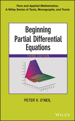
Beginning Partial Differential Equations (eBook)

Peter V. O'Neil (Autor)

eBook Download: EPUB

2014 | 3. Auflage
John Wiley & Sons (Verlag)
978-1-118-62998-7 (ISBN)

Infos

A broad introduction to PDEs with an emphasis on specialized topics and applications occurring in a variety of fields

Featuring a thoroughly revised presentation of topics, Beginning Partial Differential Equations, Third Edition provides a challenging, yet accessible, combination of techniques, applications, and introductory theory on the subjectof partial differential equations. The new edition offers nonstandard coverageon material including Burger's equation, the telegraph equation, damped wavemotion, and the use of characteristics to solve nonhomogeneous problems.

The Third Edition is organized around four themes: methods of solution for initial-boundary value problems; applications of partial differential equations; existence and properties of solutions; and the use of software to experiment with graphics and carry out computations. With a primary focus on wave and diffusion processes, Beginning Partial Differential Equations, Third Edition also includes:

• Proofs of theorems incorporated within the topical presentation, such as the existence of a solution for the Dirichlet problem
• The incorporation of Maple? to perform computations and experiments
• Unusual applications, such as Poe's pendulum
• Advanced topical coverage of special functions, such as Bessel, Legendre polynomials, and spherical harmonics
• Fourier and Laplace transform techniques to solve important problems

Beginning of Partial Differential Equations, Third Edition is an ideal textbook for upper-undergraduate and first-year graduate-level courses in analysis and applied mathematics, science, and engineering.

PETER V. O'NEIL, PHD, is Professor Emeritus in the Department of Mathematics at the University of Alabama at Birmingham. He has over forty years of experience in teaching and writing and is the recipient of the Lester R. Ford Award from the Mathematical Association of America. Dr. O'Neil is also a member of the American Mathematical Society, the Mathematical Association of America, the Society for Industrial and Applied Mathematics, and the American Association for the Advancement of Science.

Inhalt

1 First Ideas 1

1.1 Two Partial Differential Equations 1

1.2 Fourier Series 10

1.3 Two Eigenvalue Problems 28

1.4 A Proof of the Fourier Convergence Theorem 30

2. Solutions of the Heat Equation 39

2.1 Solutions on an Interval (0, L) 39

2.2 A Nonhomogeneous Problem 64

2.3 The Heat Equation in Two space Variables 71

2.4 The Weak Maximum Principle 75

3. Solutions of the Wave Equation 81

3.1 Solutions on Bounded Intervals 81

3.2 The Cauchy Problem 109

3.3 The Wave Equation in Higher Dimensions 137

4. Dirichlet and Neumann Problems 147

4.1 Laplace's Equation and Harmonic Functions 147

4.2 The Dirichlet Problem for a Rectangle 153

4.3 The Dirichlet Problem for a Disk 158

4.4 Properties of Harmonic Functions 165

4.5 The Neumann Problem 187

4.6 Poisson's Equation 197

4.7 Existence Theorem for a Dirichlet Problem 200

5. Fourier Integral Methods of Solution 213

5.1 The Fourier Integral of a Function 213

5.2 The Heat Equation on a Real Line 220

5.3 The Debate over the Age of the Earth 230

5.4 Burger's Equation 233

5.5 The Cauchy Problem for a Wave Equation 239

5.6 Laplace's Equation on Unbounded Domains 244

6. Solutions Using Eigenfunction Expansions 253

6.1 A Theory of Eigenfunction Expansions 253

6.2 Bessel Functions 266

6.3 Applications of Bessel Functions 279

6.4 Legendre Polynomials and Applications 288

7. Integral Transform Methods of Solution 307

7.1 The Fourier Transform 307

7.2 Heat and Wave Equations 318

7.3 The Telegraph Equation 332

7.4 The Laplace Transform 334

8 First-Order Equations 341

8.1 Linear First-Order Equations 342

8.2 The Significance of Characteristics 349

8.3 The Quasi-Linear Equation 354

9 End Materials 361

9.1 Notation 361

9.2 Use of MAPLE 363

9.3 Answers to Selected Problems 370

Index 434

Rezensionen

"I enjoyed perusing O'Neil's book. A beginner in the field of PDEs will learn quite a number of juicy facts concerning the flow of heat and the transmission of waves. While a next step will undoubtedly involve more rigor in the use of analytic tools, this first course will catch the attention of those with a curiosity for studying physical processes using differential equations." (Mathematical Association of America, 15 February 2015)

"This book is one of the textbooks that provide an introduction to basic methods and applications of partial differential equations for students of mathematics, physics and engineering." (Zentralblatt MATH, 1 October 2014)

Textauszug

Chapter 1

First Ideas

We will begin a study of partial differential equations by deriving equations modeling diffusion processes and wave motion. These are widely applicable in the physical and life sciences, engineering, economics, and other areas. Following this, we will lay the foundations for the Fourier method, which is used to write solutions for many kinds of problems, and then solve two eigenvalue/eigenfunction problems that occur frequently when this method is used.

The chapter concludes with a proof of a theorem on the convergence of Fourier series.

1.1 Two Partial Differential Equations

1.1.1 The Heat, or Diffusion, Equation

We will derive a partial differential equation modeling heat flow in a medium. Although we will speak in terms of heat flow because it is familiar to us, the heat equation applies to general diffusion processes, which might be a flow of energy, a dispersion of insect or bacterial populations in controlled environments, changes in the concentration of a chemical dissolving in a fluid, or many other phenomena of interest. For this reason the heat equation is also called the diffusion equation.

Consider a bar of material of constant density, ρ, having uniform cross sections with area A. The lateral surface of the bar is insulated, so there is no heat loss across this surface.

Place an x-axis along the length, L, of the bar and assume that at a given time, the temperature is the same along any cross section perpendicular to this axis, although it may vary from one cross section to another. We will derive an equation for u(x, t), the temperature in the cross section of the bar at x, at time t. In the context of diffusion, u(x, t) is called a density distribution function.

Let c be the specific heat of the material of the bar. This is the amount of heat energy that must be supplied to a unit mass of the material to raise its temperature one degree. The segment of bar between x and x + Δx has mass ρAΔx, and it will take approximately ρcAu(x, t)Δx units of heat energy to change the temperature of this segment from zero to u(x, t), its temperature at time t.

The total heat energy in this segment at any time t > 0 is

This amount of heat energy within the segment at time t can increase in two ways: heat energy may flow into the segment across its ends (this change is the flux of the energy), and/or there may be a source or loss of heat energy within the segment. This can occur if there is, say, a chemical reaction or if the material is radioactive.

The rate of change of the temperature within the segment, with respect to time, is therefore

Assume for now that there is no source or loss of energy within the bar. Then

(1.1)

Now let F(x, t) be the amount of heat energy per unit area flowing across the cross section at x at time t, in the direction of increasing x. Then the flux of the energy into the segment between x and x + Δx at time t is the rate of flow into the segment across the section at x, minus the rate of flow out of the segment across the section at x + Δx (Figure 1.1):

Figure 1.1: Flux in segment = rate in minus rate out.

Write this as

(1.2)

Now recall Newton’s law of cooling, which states that heat energy flows from the warmer to the cooler region, and the amount of heat energy is proportional to the temperature difference (gradient). This means that

The positive constant of proportionality, K, is called the heat conductivity of the bar. The negative sign in this equation is due to the fact that energy flows from the warmer to the cooler segment. Substitute this expression for F(x, t) into equation 1.2 to obtain

Write this as

(1.3)

From equations 1.1 and 1.3 for the flux, we have

Divide out the common factor A and write this equation as

This equation must be valid for any choices of x and x + Δx, as long as

If the integrand were nonzero at some x, then, assuming continuity of this integrand (which is reasonable on physical grounds), it would be nonzero, therefore strictly positive or strictly negative on some interval (x, x + Δx). This would force this integral to be positive or negative, not zero, for this x and Δx, and this is a contradiction. We conclude that the integrand must be identically zero, hence

It is convenient to denote partial derivatives using subscripts. In this notation,

(1.4)

where k = K/cρ is called the diffusivity of the material of the bar. Equation 1.4 is the one-dimensional heat, or diffusion, equation. This equation, with appropriate boundary and initial conditions, models a wide range of diffusion phenomena, providing a setting for a mathematical analysis to draw conclusions about the behavior of the process under study.

If we allow for a source term Q(x, t), then the heat equation is

(1.5)

We say that equation 1.4 is homogeneous. Because of the Q(x, t) term, equation 1.5 is nonhomogeneous. Both equations are second-order partial differential equations because they contain at least one second derivative term, but no higher derivative. Both equations are also linear, which means they are linear in the unknown function and its derivatives. By contrast, the second-order partial differential equation

is nonlinear because of the uux term, which allows for an interaction between the density function, u, and its rate of change with respect to x.

The linear, homogeneous heat equation ut = kuxx has the important features that a finite sum of solutions and a product of a solution by a constant are again solutions. That is, if u1(x, y) and u2(x, y) are solutions, then au1(x, y)+bu2(x, y) is also a solution for any numbers a and b. This can be verified by substituting au1 + bu2 into equation 1.4. This is not the case with the nonhomogeneous equation 1.5, as can also be seen by substitution.

Everyday experience suggests that to know the temperature in a bar of material at any time we have to have some information, such as the temperature throughout the bar at some particular time (this is an initial condition), together with information about the temperatures at the ends of the bar (these are boundary conditions). A typical initial condition has the form

in which f(x) is a given function. Initial is taken as time zero as a convenience.

Boundary conditions specify conditions at end points of the space variable (or perhaps on a surface in higher dimensional models). These can take different forms. One commonly seen set of boundary conditions is

where α(t) and β(t) are given functions. These specify conditions at the left and right ends of the material at all times.

Boundary conditions may also reflect other physical conditions at the boundary. We will see some of these when we solve specific problems in different settings.

A problem consisting of the heat equation, together with initial and boundary conditions, is called a initial-boundary value problem for the heat equation.

1.1.2 The Wave Equation

Imagine a string (guitar string, wire, telephone line, power line, or the like) suspended between two points. We want to describe the motion of the string if it is fixed at its ends, displaced in a specified way and released with a given velocity.

Place an x-axis along the straightened string from 0 to L, and assume that each particle of string moves only vertically in a plane. We seek a function u(x, t) so that, at any time t ≥ 0, the graph of the function u = u(x, t) gives the position or shape of the string at that time. This enables us to view snapshots of the string in motion.

Begin with a simple case by neglecting damping effects, such as air resistance and the weight of the string. Let T(x, t) be the tension in the string at point x and time t, and assume that this acts tangentially to the string. The magnitude of this vector is T(x, t) = || T(x, t) ||. Also assume that the mass, ρ, per unit length is constant.

Apply Newton’s second law of motion to the segment of string between x and x + Δx. This states that the net force on the segment due to the tension is equal to the acceleration of the center of mass of the segment times the mass of the segment. This is a vector equation, meaning that we can match the horizontal components and the vertical components of both sides. Looking at the vertical components in Figure 1.2 gives us approximately

Figure 1.2: Segment of string between x and x + Δx.

in which is the center of mass of this segment of string. Then

The vertical component, v(x, t), of the tension is

Then

Let Δx → 0. Then...

Produkt-Details

• Erscheint lt. Verlag: 7.5.2014
• Reihe/Serie: Pure and Applied Mathematics: A Wiley Series of Texts, Monographs and Tracts
• Reihe/Serie: Wiley Series in Pure and Applied Mathematics
• Reihe/Serie: Wiley Series in Pure and Applied Mathematics
• Sprache: englisch
• Themenwelt: Mathematik / Informatik ► Mathematik ► Analysis
• Themenwelt: Technik
• Schlagworte: Applied Mathematics in Engineering • Applied Mathematics in Science • Applied Mathmatics in Engineering • Beginning Partial Differential Equations • Canonical Forms • Cauchy problem • Differential Equations • Differentialgleichung • Differentialgleichungen • Dirichlet and Neumann problems • Fourier series • integrals • Laplace transform • Mathematics • Mathematik • Mathematik in den Ingenieurwissenschaften • Mathematik in den Naturwissenschaften • Partielle Differentialgleichung • Peter V. O'Neil • quasi-linear PDEs • Transforms
• ISBN-10: 1-118-62998-1 / 1118629981
• ISBN-13: 978-1-118-62998-7 / 9781118629987