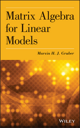
Matrix Algebra for Linear Models (eBook)

Marvin H. J. Gruber (Autor)

eBook Download: EPUB

2013
John Wiley & Sons (Verlag)
978-1-118-60881-4 (ISBN)

Infos

Matrix methods have evolved from a tool for expressing statistical problems to an indispensable part of the development, understanding, and use of various types of complex statistical analyses. This evolution has made matrix methods a vital part of statistical education. Traditionally, matrix methods are taught in courses on everything from regression analysis to stochastic processes, thus creating a fractured view of the topic. Matrix Algebra for Linear Models offers readers a unique, unified view of matrix analysis theory (where and when necessary), methods, and their applications. Written for future statisticians, both theoretical and applied, this book emphasizes the key topics that are needed in a concise and accurate way. Emphasis is on understanding and interpreting principal components as an eigenvalue, generalized inverses, and singular value decomposition. The derivation of important results in Analysis of Variance (ANOVA) is made elegant by the use of some of the properties of quadratic forms, the Kronecker product, and special matrices. A large number of numerical examples and exercises are included to further illustrate the motivation behind the concepts.

---

A self-contained introduction to matrix analysis theory and applications in the field of statistics Comprehensive in scope, Matrix Algebra for Linear Models offers a succinct summary of matrix theory and its related applications to statistics, especially linear models. The book provides a unified presentation of the mathematical properties and statistical applications of matrices in order to define and manipulate data. Written for theoretical and applied statisticians, the book utilizes multiple numerical examples to illustrate key ideas, methods, and techniques crucial to understanding matrix algebra s application in linear models. Matrix Algebra for Linear Models expertly balances concepts and methods allowing for a side-by-side presentation of matrix theory and its linear model applications. Including concise summaries on each topic, the book also features: Methods of deriving results from the properties of eigenvalues and the singular value decomposition Solutions to matrix optimization problems for obtaining more efficient biased estimators for parameters in linear regression models A section on the generalized singular value decomposition Multiple chapter exercises with selected answers to enhance understanding of the presented material Matrix Algebra for Linear Models is an ideal textbook for advanced undergraduate and graduate-level courses on statistics, matrices, and linear algebra. The book is also an excellent reference for statisticians, engineers, economists, and readers interested in the linear statistical model.

Autor

MARVIN H. J. GRUBER, PHD, is Professor Emeritus in the School of Mathematical Sciences at Rochester Institute of Technology. He has authored several books and journal articles in his areas of research interest, which include improving the efficiency of regression estimators. Dr. Gruber is a member of the American Mathematical Society and the American Statistical Association.

Rezensionen

"This book seems suitable for an advanced undergraduate and/or introductory master's level course . . . Four appealing features of this book are its inclusion of an overview, a summary, exercises (with answers provided), and numerical examples for all sections." (American Mathematical Society, 1 November 2015)

"The book is suitable for graduate and postgraduate students and researchers. This book is highly recommended." (Zentralblatt, 1 April 2015)

"This is an excellent and comprehensive presentation of the use of matrices for linear models. The writing is very clear, and the layout is excellent. It would serve well either as a class text or as the foundation for individual personal study." (International Statistical Review, 18 March 2014)

Textauszug

SECTION 1

WHAT MATRICES ARE AND SOME BASIC OPERATIONS WITH THEM

1.1 INTRODUCTION

This section will introduce matrices and show how they are useful to represent data. It will review some basic matrix operations including matrix addition and multiplication. Some examples to illustrate why they are interesting and important for statistical applications will be given. The representation of a linear model using matrices will be shown.

1.2 WHAT ARE MATRICES AND WHY ARE THEY INTERESTING TO A STATISTICIAN?

Matrices are rectangular arrays of numbers. Some examples of such arrays are

Often data may be represented conveniently by a matrix. We give an example to illustrate how.

 

Example 1.1 Representing Data by Matrices

An example that lends itself to statistical analysis is taken from the Economic Report of the President of the United States in 1988. The data represent the relationship between a dependent variable Y (personal consumption expenditures) and three other independent variables X1, X2, and X3. The variable X1 represents the gross national product, X2 represents personal income (in billions of dollars), and X3 represents the total number of employed people in the civilian labor force (in thousands). Consider this data for the years 1970–1974 in Table 1.1.

TABLE 1.1 Consumption expenditures in terms of gross national product, personal income, and total number of employed people

The dependent variable may be represented by a matrix with five rows and one column. The independent variables could be represented by a matrix with five rows and three columns. Thus,

A matrix with m rows and n columns is an m × n matrix. Thus, the matrix Y in Example 1.1 is 5 × 1 and the matrix X is 5 × 3. A square matrix is one that has the same number of rows and columns. The individual numbers in a matrix are called the elements of the matrix.  

We now give an example of an application from probability theory that uses matrices.

 

Example 1.2 A “Musical Room” Problem

Another somewhat different example is the following. Consider a triangular-shaped building with four rooms one at the center, room 0, and three rooms around it numbered 1, 2, and 3 clockwise (Fig. 1.1).

There is a door from room 0 to rooms 1, 2, and 3 and doors connecting rooms 1 and 2, 2 and 3, and 3 and 1. There is a person in the building. The room that he/she is in is the state of the system. At fixed intervals of time, he/she rolls a die. If he/she is in room 0 and the outcome is 1 or 2, he/she goes to room 1. If the outcome is 3 or 4, he/she goes to room 2. If the outcome is 5 or 6, he/she goes to room 3. If the person is in room 1, 2, or 3 and the outcome is 1 or 2, he/she advances one room in the clockwise direction. If the outcome is 3 or 4, he/she advances one room in the counterclockwise direction. An outcome of 5 or 6 will cause the person to return to room 0. Assume the die is fair.

FIGURE 1.1 Building with four rooms.

Let pij be the probability that the person goes from room i to room j. Then we have the table of transitions

that indicates

Then the transition matrix would be

  

Matrices turn out to be handy for representing data. Equations involving matrices are often used to study the relationship between variables.

More explanation of how this is done will be offered in the sections of the book that follow.

The matrices to be studied in this book will have elements that are real numbers. This will suffice for the study of linear models and many other topics in statistics. We will not consider matrices whose elements are complex numbers or elements of an arbitrary ring or field.

We now consider some basic operations using matrices.

1.3 MATRIX NOTATION, ADDITION, AND MULTIPLICATION

We will show how to represent a matrix and how to add and multiply two matrices.

The elements of a matrix A are denoted by aij meaning the element in the ith row and the jth column. For example, for the matrix

c11 = 0.2, c12 = 0.5, and so on. Three important operations include matrix addition, multiplication of a matrix by a scalar, and matrix multiplication. Two matrices A and B can be added only when they have the same number of rows and columns. For the matrix C = A + B, cij = aij + bij; in other words, just add the elements algebraically in the same row and column. The matrix D = αA where α is a real number has elements dij = αaij; just multiply each element by the scalar. Two matrices can be multiplied only when the number of columns of the first matrix is the same as the number of rows of the second one in the product. The elements of the n × p matrix E = AB, assuming that A is n × m and B is m × p, are

 

Example 1.3 Illustration of Matrix Operations

Let .

Then

and

  

 

Example 1.4 Continuation of Example 1.2

Suppose that elements of the row vector where represent the probability that the person starts in room i. Then π(1) = π(0)P. For example, if

the probabilities the person is in room 0 initially are 1/2, room 1 1/6, room 2 1/12, and room 3 1/4, then

Thus, after one transition given the initial probability vector above the probabilities that the person ends up in room 0, room 1, room 2, or room 3 after one transition are 1/6, 5/18, 11/36, and 1/4, respectively. This example illustrates a discrete Markov chain. The possible transitions are represented as elements of a matrix.

Suppose we want to know the probabilities that a person goes from room i to room j after two transitions. Assuming that what happens at each transition is independent, we could multiply the two matrices. Then

Thus, for example, if the person is in room 1, the probability that he/she returns there after two transitions is 1/3. The probability that he/she winds up in room 3 is 2/9. Also when π(0) is the initial probability vector, we have that π(2) = π(1)P = π(0)P2. The reader is asked to find π(2) in Exercise 1.17.  

Two matrices are equal if and only if their corresponding elements are equal. More formally, A = B if and only if aij = bij for all 1 ≤ i ≤ m and 1 ≤ j ≤ n.

Most, but not all, of the rules for addition and multiplication of real numbers hold true for matrices. The associative and commutative laws hold true for addition. The zero matrix is the matrix with all of the elements zero. An additive inverse of a matrix A would be −A, the matrix whose elements are (−1)aij. The distributive laws hold true.

However, there are several properties of real numbers that do not hold true for matrices. First, it is possible to have divisors of zero. It is not hard to find matrices A and B where AB = 0 and neither A or B is the zero matrix (see Example 1.4).

In addition the cancellation rule does not hold true. For real nonzero numbers a, b, c, ba = ca would imply that b = c. However (see Example 1.5) for matrices, BA = CA may not imply that B = C.

Not every matrix has a multiplicative inverse. The identity matrix denoted by I has all ones on the longest (main) diagonal (aij = 1) and zeros elsewhere (aij = 0, i ≠ j). For a matrix A, a multiplicative inverse would be a matrix such that AB = I and BA = I. Furthermore, for matrices A and B, it is not often true that AB = BA. In other words, matrices do not satisfy the commutative law of multiplication in general.

The transpose of a matrix A is the matrix A′ where the rows and the columns of A are exchanged. For example, for the matrix A in Example 1.3,

A matrix A is symmetric when A = A′. If A = − A′, the matrix is said to be skew symmetric. Symmetric matrices come up often in statistics.

 

Example 1.5 Two Nonzero Matrices Whose Product Is Zero

Consider the matrix

Notice that

  

 

Example 1.6 The Cancellation Law for Real Numbers Does Not Hold for Matrices

Consider matrices A, B, C where

Now

but B ≠ C.  

Matrix theory is basic to the study of linear models. Example 1.7 indicates how the basic matrix operations studied so far are used in this context.

 

Example 1.7 The Linear Model

Let Y be an n-dimensional vector of observations, an n × 1 matrix. Let X be an n × m matrix where each column has the values of a prediction variable. It is assumed here that there are m predictors. Let β be an m × 1 matrix of parameters to be estimated. The prediction of the observations will not be exact. Thus, we also need an n-dimensional column vector of errors ε. The general linear model will take the form

(1.1)  

Suppose that there are five observations and three prediction variables. Then n = 5 and m = 3. As a result, we would have the multiple regression equation

(1.2)  

Equation (1.2) may be represented by the matrix equation

(1.3)  

In experimental design models, the matrix is frequently zeros and ones indicating the level of a factor. An example of such a model would be

(1.4)  

This is an unbalanced one-way analysis of variance (ANOVA) model where there are three treatments with four observations of treatment 1, three observations of treatment 2, and two observations of treatment 3....

Produkt-Details

• Erscheint lt. Verlag: 13.12.2013
• Sprache: englisch
• Themenwelt: Mathematik / Informatik ► Mathematik ► Algebra
• Themenwelt: Mathematik / Informatik ► Mathematik ► Statistik
• Themenwelt: Mathematik / Informatik ► Mathematik ► Wahrscheinlichkeit / Kombinatorik
• Themenwelt: Technik
• Schlagworte: Algebra • Analysis • Angew. Wahrscheinlichkeitsrechn. u. Statistik / Modelle • Applications • Applied Probability & Statistics - Models • Book • Comprehensive • Field • Introduction • Linear • linear algebra • Lineare Algebra • Mathematical • Mathematics • Mathematik • matrices • Matrix • Models • Order • Properties • Scope • selfcontained • Statistical • Statistics • Statistik • succinct • Summary • theory
• ISBN-10: 1-118-60881-X / 111860881X
• ISBN-13: 978-1-118-60881-4 / 9781118608814