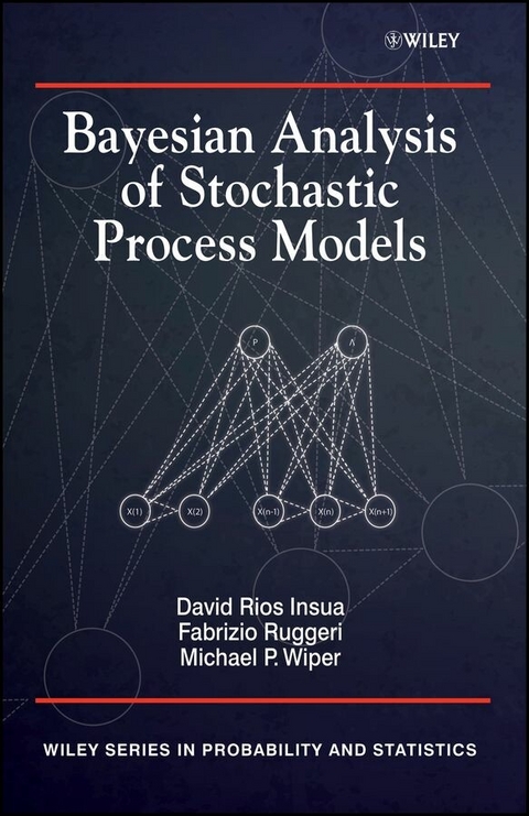
Bayesian Analysis of Stochastic Process Models (eBook)

David Insua, Fabrizio Ruggeri, Mike Wiper (Autoren)

eBook Download: EPUB

2012
John Wiley & Sons (Verlag)
978-1-118-30403-7 (ISBN)

Infos

Bayesian analysis of complex models based on stochastic processes has in recent years become a growing area. This book provides a unified treatment of Bayesian analysis of models based on stochastic processes, covering the main classes of stochastic processing including modeling, computational, inference, forecasting, decision making and important applied models.

Key features:

• Explores Bayesian analysis of models based on stochastic processes, providing a unified treatment.
• Provides a thorough introduction for research students.
• Computational tools to deal with complex problems are illustrated along with real life case studies
• Looks at inference, prediction and decision making.

Researchers, graduate and advanced undergraduate students interested in stochastic processes in fields such as statistics, operations research (OR), engineering, finance, economics, computer science and Bayesian analysis will benefit from reading this book. With numerous applications included, practitioners of OR, stochastic modelling and applied statistics will also find this book useful.

Autor

Fabrizio Ruggeri, Research Director, CNR IMATI, Milano, Italy. Michael P. Wiper, Associate Professor in Statistics, Department of Statistics, Universidad Carlos III de Madrid, Spain. David Rios Insua, Professor of Statistics and Operations Research, Department of Statistics and Operations Research, Universidad Rey Juan Carlos, Spain.

Inhalt

Preface

PART ONE BASIC CONCEPTS AND TOOLS

1 Stochastic Processes 11

1.1 Introduction 11

1.2 Key Concepts in Stochastic Processes 11

1.3 Main Classes of Stochastic Processes 16

1.4 Inference, Prediction and Decision Making 21

1.5 Discussion 23

2 Bayesian Analysis 27

2.1 Introduction 27

2.2 Bayesian Statistics 28

2.3 Bayesian Decision Analysis 37

2.4 Bayesian Computation 39

2.5 Discussion 51

PART TWO MODELS

3 Discrete Time Markov Chains 61

3.1 Introduction 61

3.2 Important Markov Chain Models 62

3.3 Inference for First Order Chains 66

3.4 Special Topics 76

3.5 Case Study: Wind Directions at Gijon 87

3.6 Markov Decision Processes 94

3.7 Discussion 97

4 Continuous Time Markov Chains and Extensions 105

4.1 Introduction 105

4.2 Basic Setup and Results 106

4.3 Inference and Prediction for CTMCs 108

4.4 Case Study: Hardware Availability through CTMCs 112

4.5 Semi-Markovian Processes 118

4.6 Decision Making with Semi-Markovian Decision Processes
122

4.7 Discussion 128

5 Poisson Processes and Extensions 133

5.1 Introduction 133

5.2 Basics on Poisson Processes 134

5.3 Homogeneous Poisson Processes 138

5.4 Nonhomogeneous Poisson Processes 147

5.5 Compound Poisson Processes 153

5.6 Further Extensions of Poisson Processes 154

5.7 Case Study: Earthquake Occurrences 157

5.8 Discussion 162

6 Continuous Time Continuous Space Processes 169

6.1 Introduction 169

6.2 Gaussian Processes 170

6.3 Brownian Motion and Fractional Brownian Motion 174

6.4 Di®usions 181

6.5 Case Study: Prey-predator Systems 184

6.6 Discussion 190

PART THREE APPLICATIONS

7 Queueing Analysis 201

7.1 Introduction 201

7.2 Basic Queueing Concepts 201

7.3 The Main Queueing Models 204

7.4 Inference for Queueing Systems 208

7.5 Inference for M=M=1 Systems 209

7.6 Inference for Non Markovian Systems 220

7.7 Decision Problems in Queueing Systems 229

7.8 Case Study: Optimal Number of Beds in a Hospital 230

7.9 Discussion 235

8 Reliability 245

8.1 Introduction 245

8.2 Basic Reliability Concepts 246

8.3 Renewal Processes 249

8.4 Poisson Processes 251

8.5 Other Processes 259

8.6 Maintenance 262

8.7 Case Study: Gas Escapes 263

8.8 Discussion 271

9 Discrete Event Simulation 279

9.1 Introduction 279

9.2 Discrete Event Simulation Methods 280

9.3 A Bayesian View of DES 283

9.4 Case Study: A G=G=1 Queueing System 286

9.5 Bayesian Output Analysis 288

9.6 Simulation and Optimization 292

9.7 Discussion 294

10 Risk Analysis 301

10.1 Introduction 301

10.2 Risk Measures 302

10.3 Ruin Problems 316

10.4 Case Study: Ruin Probability Estimation 320

10.5 Discussion 327

Appendix A Main Distributions 337

Appendix B Generating Functions and the Laplace-Stieltjes
Transform 347

Index

Textauszug

1

Stochastic processes

1.1 Introduction

The theme of this book is Bayesian Analysis of Stochastic Process Models. In this first chapter, we shall provide the basic concepts needed in defining and analyzing stochastic processes. In particular, we shall review what stochastic processes are, their most important characteristics, the important classes of processes that shall be analyzed in later chapters, and the main inference and decision-making tasks that we shall be facing. We also set up the basic notation that will be followed in the rest of the book. This treatment is necessarily brief, as we cover material which is well known from, for example, the texts that we provide in our final discussion.

1.2 Key concepts in stochastic processes

Stochastic processes model systems that evolve randomly in time, space or space-time. This evolution will be described through an index . Consider a random experiment with sample space Ω, endowed with a σ-algebra and a base probability measure P. Associating numerical values with the elements of that space, we may define a family of random variables , which will be a stochastic process. This idea is formalized in our first definition that covers our object of interest in this book.

Definition 1.1: A stochastic process is a collection of random variables Xt, indexed by a set T, taking values in a common measurable space S endowed with an appropriate σ-algebra.

T could be a set of times, when we have a temporal stochastic process; a set of spatial coordinates, when we have a spatial process; or a set of both time and spatial coordinates, when we deal with a spatio-temporal process. In this book, in general, we shall focus on stochastic processes indexed by time, and will call T the space of times. When T is discrete, we shall say that the process is in discrete time and will denote time through n and represent the process through When T is continuous, we shall say that the process is in continuous time. We shall usually assume that in this case. The values adopted by the process will be called the states of the process and will belong to the state space S. Again, S may be either discrete or continuous.

At least two visions of a stochastic process can be given. First, for each we may rewrite and we have a function of t which is a realization or a sample function of the stochastic process and describes a possible evolution of the process through time. Second, for any given t, Xt is a random variable. To completely describe the stochastic process, we need a joint description of the family of random variables , not just the individual random variables. To do this, we may provide a description based on the joint distribution of the random variables at any discrete subset of times, that is, for any with and for any we provide

Appropriate consistency conditions over these finite-dimensional families of distributions will ensure the definition of the stochastic process, via the Kolmogorov extension theorem, as in, for example, Øksendal (2003).

Theorem 1.1: Let . Suppose that, for any with the random variables satisfy the following consistency conditions:

1. For all permutations of and we have that

2. For all and , we have .

Then, there exists a probability space and a stochastic process having the families as finite-dimensional distributions.

Clearly, the simplest case will hold when these random variables are independent, but this is the territory of standard inference and decision analysis. Stochastic processes adopt their special characteristics when these variables are dependent.

Much as with moments for standard distributions, we shall use some tools to summarize a stochastic process. The most relevant are, assuming all the involved moments exist:

Definition 1.2: For a given stochastic process the mean function is

The autocorrelation function of the process is the function

Finally, the autocovariance function of the process is

It should be noted that these moments are merely summaries of the stochastic process and do not characterize it, in general.

An important concept is that of a stationary process, that is a process whose characterization is independent of the time at which the observation of the process is initiated.

Definition 1.3: We say that the stochastic process is strictly stationary if for any n, and τ, () has the same distribution as

A process which does not satisfy the conditions of Definition 1.3 will be called nonstationary. Stationarity is a typical feature of a system which has been running for a long time and has stabilized its behavior.

The required condition of equal joint distributions in Definition 1.3 has important parameterization implications when n=1, 2. In the first case, we have that all Xt variables have the same common distribution, independent of time. In the second case, we have that the joint distribution depends on the time differences between the chosen times, but not on the particular times chosen, that is,

Therefore, we easily see the following.

Proposition 1.1: For a strictly stationary stochastic process , the mean function is constant, that is,

(1.1)

Also, the autocorrelation function of the process is a function of the time differences, that is,

(1.2)

Finally, the autocovariance function is given by

assuming all relevant moments exist.

A process that fulfills conditions (1.1) and (1.2) is commonly known as a weakly stationary process. Such a process is not necessarily strictly stationary, whereas a strictly stationary process will be weakly stationary if first and second moments exist.

Example 1.1: A first-order autoregressive, or AR(1), process is defined through

where is a sequence of independent and identically distributed (IID) normal random variables with zero mean and variance . This process is weakly, but not strictly, stationary if . Then, we have which implies that If the process is not stationary.

When dealing with a stochastic process, we shall sometimes be interested in its transition behavior, that is, given some observations of the process, we aim at forecasting some of its properties a certain time t ahead in the future. To do this, it is important to provide the so called transition functions. These are the conditional probability distributions based on the available information about the process, relative to a specific value of the parameter t0.

Definition 1.4: Let be such that The conditional transition distribution function is defined by

When the process is discrete in time and space, we shall use the transition probabilities defined, for through

When the process is stationary, the transition distribution function will depend only on the time differences

For convenience, the previous expression will sometimes be written as Analogously, for the discrete process we shall use the expression

Letting we may consider the long-term limiting behavior of the process, typically associated with the stationary distribution. When this distribution exists, computations are usually much simpler than doing short-term predictions based on the use of the transition functions. These limit distributions reflect a parallelism with the laws of large numbers, for the case of IID observations, in that

when for some limiting random variable This is the terrain of ergodic theorems and ergodic processes, see, e.g., Walters (2000).

In particular, for a given stochastic process, we may be interested in studying the so-called time averages. For example, we may define the mean time average, which is the random variable defined by

If the process is stationary, interchanging expectation with integration, we have

This motivates the following definition.

Definition 1.5: The process Xt is said to be mean ergodic if:

1. for some and

2.

An autocovariance ergodic process can be defined in a similar way. Clearly, for a stochastic process to be ergodic, it has to be stationary. The converse is not true.

1.3 Main classes of stochastic processes

Here, we define the main types of stochastic processes that we shall study in this book. We start with Markov chains and Markov processes, which will serve as a model for many of the other processes analyzed in later chapters and are studied in detail in Chapters 3 and 4.

1.3.1 Markovian processes

Except for the case of independence, the simplest dependence form among the random variables in a stochastic process is the Markovian one.

Definition 1.6: Consider a set of time instants with and . A stochastic process is Markovian if the distribution of Xt conditional on the values of depends only on that is, the most recent known value of the process

(1.3)

As a...

Produkt-Details

• Erscheint lt. Verlag: 2.4.2012
• Reihe/Serie: Wiley Series in Probability and Statistics
• Reihe/Serie: Wiley Series in Probability and Statistics
• Reihe/Serie: Wiley Series in Probability and Statistics
• Sprache: englisch
• Themenwelt: Mathematik / Informatik ► Mathematik ► Statistik
• Themenwelt: Mathematik / Informatik ► Mathematik ► Wahrscheinlichkeit / Kombinatorik
• Themenwelt: Technik
• Schlagworte: Activity • Analysis • Bayesian • Bayesian analysis • Bayessches Verfahren • Bayes-Verfahren • Complex • Engineering statistics • Experimental Design • important • Main • Models • models explores • Process • processes • Processing • Research • Statistics • Statistik • Statistik in den Ingenieurwissenschaften • stochastic • surge • Treatment • Unified • Versuchsplanung • years
• ISBN-10: 1-118-30403-9 / 1118304039
• ISBN-13: 978-1-118-30403-7 / 9781118304037